Random Variation Vs Trends
Understanding variation is key to interpret the value stream behavior. Not all variation is the same.
Variation

These are some factors which may add variation to the process of cooking a turkey.
Every process has variation. Some causes of variation may be identified and acted upon.We can use two metrics for variation which complement each other:

Manual Dice Throwing
This simple exercise can help to experience process variation and understand the difference between a process change and inherent process variation.This understanding is key on management decisions to avoid both overreaction and lack of reaction.
To run the exercise with actual dice print the form:

Exercise:
- You will need a printed form and 4 dice for each team
- Throw 4 dice and add the outcomes
- Record the result in the Run Chart
- Repeat 50 times
- Join the dots in the Run Chart with a line
- Build the Histogram by counting the total number of dots on each group of 3 values
Run this Exercise with a Simulator
Download this Excel file Variation.xlsm to your PC from OneDriveClose all Excel sheets before you open this one and enable MACROS.

Results Interpretation Questions:
Try to answer these questions on each team and then discuss all teams together:
- Does each outcome depend on the previous one?
- Are there any special trends or indication of process change in the run chart? Is this a stable process?
- Is there a special cause that explains the maximum and the minimum values? Did you do anything different to obtain them?
- If we have a target to achieve the maximum possible value will motivation from management help?
- Is the frequency distribution close to normal: maximum at the center, declining frequency on both sides, symmetrical?
- What distribution would result throwing one single die? Why?
- Is it possible to predict the outcome of one specific throw?
- Is it possible to predict the frequency of one specific outcome for a large number of throws?
- Can two different run charts produce the same histogram
Answers:
- If a number won last year it has less chance than other numbers this year.
- After 3 consecutive reds there is more chance of getting a black
2. We can't see any significant trends up or down, therefore this is a stable process: it continues to behave the same way. It is stable in spite of its large variation.
This is what we would expect since we have not changed the way we throw the dice so the process will continue to behave this way while we do so.
3. We did nothing different to obtain the high or the low values: the outcomes are purely random
4. Motivation will only produce frustration of the employee and no improvement in this case. The outcome in this case is purely random and the employee running this process has no way to improve it.
Some managers, in a case like this, may get the impression that the variation is a consequence of their own positive or negative employee motivation actions, but we know, in this case, it has nothing to do with it.
5. Yes, the histogram is close to normal:

Throwing 4 dice there is only one combination that gives a sum of 4 (all 1's) but there are many combinations that give a sum of 14. The distribution of sums of 4 throws follows a normal distribution in spite of the distribution of single values following a uniform distribution (Central limit theorem)
6. One die distribution: Uniform (all outcomes have the same probability)

7. It is not possible to predict any one outcome.
8. Yes, in this case of a stable process we can know the frequency of each outcome with the histogram above for a large number of throws.
9. Yes, two different run charts can produce the same histogram. The histogram can not tell us if the process is stable. This can be done with the run chart.
Stability doesn't necessarily mean that the process is OK: it just means that the process is neither improving nor getting worse.
Alternative process
Let's now analyse another process: Open Variation.xlsm sheet ALT, press RESET and keep pressing F9 to run the process.
- Is this a stable process? Why?
- Is it likely that this data comes from the previous process of throwing 4 dice? Why?
- Can we use the frequency distribution histogram to predict process behavior in this case?
- What is the probability that values 7 - 13 happen again? Can you conclude that by looking at the histogram?
- What is the meaning of the frequency distribution histogram in this case?
Alternative Process Conclusions
1. We can clearly notice that this process has a significant upward trend, therefore it isn't a stable process: its average is shifting up.
2. Therefore it is very unlikely that it comes from throwing dice (apart from the values above 24 impossible with 4 dice).
3. In this case of an unstable process, as shown by the Run Chart, the Histogram is completely misleading if we want to predict the process behavior.
4. The histogram predicts that values below 15 have a certain probability of occurring but from the Run Chart we see that this is very unlikely.
5. If the process is not stable, as shown by the run chart, the histogram is useless to predict future behavior.
We can conclude that the Run Chart and the Histogram are both necessary and they complement each other.
First we must check that the process is stable with the Run Chart and only if it is we can use the Histogram to characterize the process behavior.
Statistical Process Control (SPC)
The question is how do we know if the process is stable (apart from just our impression)? What is a significant trend? The answer is to use an SPC chart (sheet Alt SPC):
The green and red dots indicate a significant upward trend, therefore this is not a stable process.
If it isn't stable we can't forecast how the process will behave in the future and our histogram is obviously useless.
Defect Rate Comparisons
Open Variation.xlsm sheet Defects
These are the defect rates produced by 6 operators during one week.
If you were the department manager you should decide, based on this data, whether to take some actions such as:
- Talk to Amparo to remind her of our zero defects commitment with the customer
- Congratulate Fernando for his results and, maybe, give him a prize
- Ask the process engineer to explain why Mondays produce more defects than Fridays
- Tell operators that anyone producing above 8% weekly average defects will be penalized
Corrective Actions Analysis
If you have decided on any of those actions you are wrong. In fact, they may be counter productive.This would be an example of overreaction on the part of management due to a lack of understanding of process variation.
To see this just press F9 to simulate another week with this same process: your opinion on who is best or worst may change.
If we analyse the results of 4 weeks we notice that the differences among operators aren't that large

How do we know if there is a statistically significant difference among the different operators or days of the week?
This analysis can be done with Data Analysis in Excel: 2 Factor Anova

Process Control
Open Variation.xlsm sheet Control and press Reset- You have been made responsible to control a machine to insure the deviation from target is zero in every run
- You can set the adjustment value (positive or negative) to be applied to the next run
- Set the adjustment and press F9 for the next run
- Repeat for 25 runs

Analysis of Results
- Did you achieve your objectives of controlling the process to obtain zero deviation in every run?
- Why?
- What strategy did you follow?
- What could you have done differently?
- Can you be held responsible for these results?
- Why?


Before we start making adjustments we should have seen how the process behaves with no adjustments:
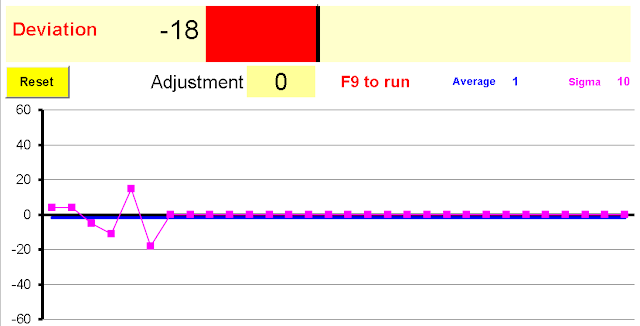
We see that the process has random variation and its average deviation is well centered in zero: this means we can't improve it with our adjustments, in fact, we will increase the variation and make it worse.
In this case the operator has been given an impossible task.
Adjusting the site after every shot: Over-reaction

Conclusions
- An understanding of process variation is essential in order to take the right improvement actions
- Decisions based on one single outcome can lead to overreaction and making the process worse
- A slow trend may pass unnoticed causing process degradation until it is too late.
- Statistical analysis is required to distinguish between a change in the process and intrinsic process variation
- Statistical applications such as Excel Data Analysis Tools can help in this analysis
- Six Sigma education for professionals and management can be useful to adopt this new way of thinking
- Real Time SPC is a useful tool to control critical process factors
- To find out which are the critical factors and their optimal values to improve the process you can use Design Of Experiments


Comments
Post a Comment