Natural gas demand is highly seasonal, therefore forecasting the final consumption is essential to manage the complete supply chain.
Temperature is a main factor affecting home gas consumption for heating.
We will analyse the correlation between gas consumption and temperature.
Download this Excel file with examples to your PC from OneDrive: Gas Forecast.xlsx
This chart of local consumption during a winter month, leads us to believe that one main factor in consumption is ambient temperature. This may be due to its wide use for heating.
We can think of other factors that may affect consumption such as the day of the week so we will analyse this actual consumption data with these two possible factors.
We obtain the day of the week with an Excel formula from the date.
We can get the average temperatures of the corresponding geographical area during this period from AEMET (Agencia Estatal de Meteorología) in aemet.es
Day of the Week Calculation
We
obtain the day of the week with this Excel formula from the date.
Regression Analysis with Excel
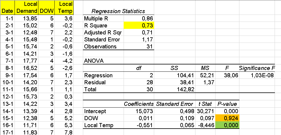
We will use Excel Data Analysis to compute the Regression with output Consumption and inputs Day of the Week (DOW) and Local Temperature as shown:
The analysis result is:
We can see a significant regression as shown by R Square of 73%. This means that 73% of the variation observed in gas consumption is due to these factors and in fact just temperature.
Looking at the two factors we notice that the p value for DOW is 0.92 which means it doesn't affect consumption: there is no significant differences in the consumption of the seven days of the week.
On the other hand a p value of zero for Local Temperature means a very significant influence in consumption.
Remove Non - significant Factors
We will now run the Regression analysis removing DOW:
Since we now have one single factor we are asking Excel to provide Residuals, Residual Plots and Line Fit Plots.
The result is:
The resulting formula is therefore: Consumption = 15.11 - 0.55 * Temperature
This is telling us there is a linear relationship between temperature and consumption which will enable us to forecast consumption based on temperature forecast from AEMET.
We notice that -0.55 means that the slope of the straight line is negative. This means that the higher the temperature the lower gas consumption. This is what we would expect.
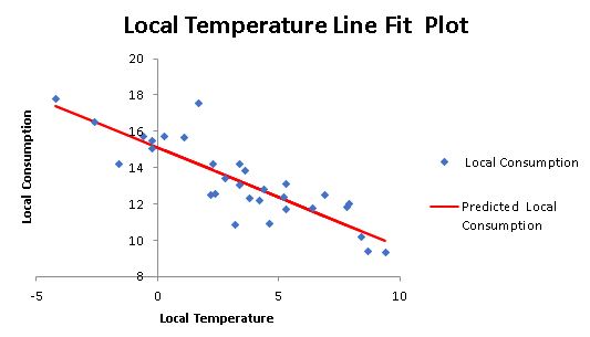
Graphically:
Here we compare the actual values with the predicted values using our previous formula: matching is quite good.
Residuals Analysis
Looking at the line fit plot we notice the actual values differ from the predicted values represented by the straight line.
The differences between the actual and predicted values (absolute values) are the residuals.
In order to validate this mathematical model we need to check that the residuals meet certain conditions.
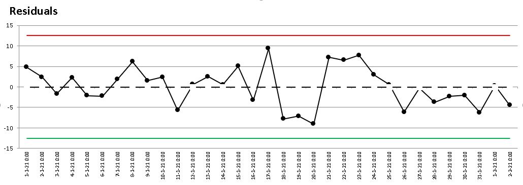
The first condition is that residuals are stable along time. We will check that with an Individuals SPC chart:
We see no out-of-control symptoms so it meets this condition.
Residuals Vs Temperature:
We check for trends in the residuals along the temperature range: No trends are detected.
Residuals Normality
Another condition is that the average of the residuals is close to zero and they follow a normal distribution:
We notice the average is zero and the p value of the Anderson Darling Normality Test is 0.87 (well above 0.05) so it is normal.
This validates our mathematical model.
Forecast
To forecast consumption in this geographic area we obtain the temperature forecast for that area from AEMET:
Applying the formula to the average temperatures we obtain the gas consumption forecast for the next 7 days.
Forecast for Other Geographic Areas
Different areas have different climats, therefore the use of gas heating is different.
This regression calculation needs to be done for each specific geographic area.
The example used so far was for a northern area and the regression equation was:
Consumption = 15.11 - 0.55 * Temperature
This equation for a central area was:
Consumption = 43.26 - 1.84 * Temperature
Differences may be due not only to temperature but also to type of consumer mix in the area: industrial, homes with gas heating, homes with no gas heating, etc.
Additional Factors Affecting this Correlation
This article analyzes other possible factors affecting the Gas consumption Vs Temperature correlation.
Summer and Winter Correlation Factors
We notice a significant correlation coefficient difference between summer ( -0.68) and winter (-0.83).
In this month of August there seems to be no correlation because the temperature never dropped below 15ºC which means homes did not turn on the heating.
There seems to be a threshold around this temperature where heating starts to be used.
Day and Night Correlation Factors
There are significant correlation coefficient differences between night and day. But this could be due to the nights being cooler than days.
Conclusions
- Final gas consumption is highly dependent on ambient temperature
- National temperature measurements can be used to calculate a regression equation for each geographic area based on the historical gas consumption in the area
- These regression formulas enable a gas consumption forecast for each area based on the weather forecast
- The regression formulas need to be recalculated when there is a major change in the different areas or at the international level.
- This correlation seems to hold as long as temperature is below a certain threshold when homes start to use heating.


Comments
Post a Comment