Design of Experiments (DOE) with Excel

Design of Experiments (DOE) is a very useful process improvement methodology. 

Microsoft Excel has some powerful data analysis tools, which I have, successfully, used for DOE.

When it comes to analyzing cause and effect, we want to know what process factors affect our outputs.

 Correlation and Regression could give us an indication of the main factors, and the extent they affect the outputs.

In some cases, there may be interactions among the different factors, or the mathematical relation between factors and outputs may not be linear.

In these cases, it is useful to run a systematic set of experiments, to test all possible combinations of factors, to relate them to the outputs.

Factorial Experiment Example

We want to minimize process loss, and after some brainstorming among the process specialists, we concluded that 5 factors may affect loss. Based on current factor levels, we have selected the following levels to experiment with:  

Download this Excel file DOE_with_Excel.xlsm from OneDrive

Factorial Designs

Full factorial designs, are constructed simply counting in binary, to obtain all the different combinations of 0 and 1, for all factors. In our designs, we just replace 0 with -1, to meet the balance property.

See sheet Designs:

1/2 Fraction Design

See sheet Half fraction:

With our 5 factors, to run a full factorial set of experiments, we would need 2 ^ 5 = 32 experiments. 

This could involve time and money, before we are sure that all factors really affect our process. 

Therefore we might start with a subset, of the full factorial, as a detection experiment. 

A 1/2 fraction will involve 1/2 the number of experiments: 16.

We can build a 1/2 fraction, 5 factor design, from a 4 factor full factorial:

  

We do this, by replacing the 4 factor interaction (which is very unlikely to happen) with the 5th factor (Flow). We construct, therefore, the Flow column, multiplying the other 4 columns.

 

Run the Experiments

To run the experiments you need to convert the coded values to uncoded as seen in sheet Run experiments:

We don't want the order in which we run the experiments affect the result, so a common practice is to randomize this order. 

To randomize the order in which to run the experiments use a macro pressing Ctrl + r and then follow the order indicated in column M:

Experiments Simulation

In this example, we are going to use a simulator, with the coded values, to simulate the running of  our experiments. See the Experiments simulation sheet:

  

We have added 2 additional experiments, with the values called central points (all zeros) which will correspond (in uncoded values) to the average value of the high and low levels, in each factor.

We do this, to make a more robust design, without going all the way to the full 32 experiments.

The simulator has provided the process loss estimation outputs, for each experiment.

In the simulator, every time we press F9, a new set of experiments is run, giving (as in real life) different results. 

  

Factor Interactions

We want to be able to estimate the influence of each individual factor in the result, but also the interactions among them, so before we analyze the results we will build a column for each interaction among 2 factors. 

If we wanted to include 3 factor interactions we would also add them to this matrix.

Sheet Detection:

  

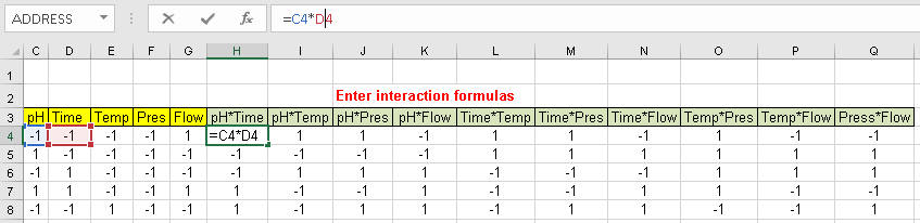
You obtain each interaction column, just by multiplying the corresponding factor columns. Just enter the formula in the first line, and replicate all the way down.

Regression with Excel Data Analysis

Enter in Excel: Data/ Data Analysis/ Regression

Fill in the regression form as shown

"Y" is the output (Loss)

"X" is the input matrix including the 5 factors and all the interactions 

And the result will be:

We notice that R^2 = 0.90 which validates our mathematical model.

The Probability column of the coefficients (p) tells us which factors and interactions are significant: those below 0.05.

Factors Temp and Press have a p value above 0.05 but their interaction is below (0.02) therefore we must keep them.

We run the Regression again keeping only the factors and interactions not removed (sheet Reduced model):

These are the results of the reduced model.

Out of the 5 original factors, which we thought could affect the output,  we have confirmed that only three affect: pH, Temp and Press. 

Temp and Press do not, significantly, affect but their interaction does. 

From the Coefficients column we will build the mathematical formula to estimate Loss as a function of these three factors. 

This gives us the formula for the estimation of Process Loss as a function of 3 factors:

Loss = 20.24 + 6.85 pH -1.4 Temp - 0.06 Pres + 4.41 Temp * Pres

This equation is with factors in coded values.

 

Process Optimization

We now want to calculate, with this mathematical model of our process, which are the pH, Temp and Pres values which will minimize Process Loss.

In order to do this we will use Excel Solver.  (See Theory of Constraints )

In the Reduced Model sheet we add cells M17:M21 to house the results we are looking for. 

M17 is the factor to multiply with the interception so it must be 1. 

Cell M21 should have the product Temp*Pres so we input the formula (=M19*M20).

We will ask Solver to give us the values for the yellow cells.

In M23 we put the formula to calculate loss with the coefficients in column I: 

                             (=SUMPRODUCT(I17:I21;M17:M21)

We now call Solver to minimize this value in M23, changing pH, Temp and Pres with the restrictions that they must be between -1 and +1.

Solver gives us these results: the optimal values of pH, Temp and Pres, to obtain a minimum loss of 7.64

The result is that the minimum loss of 7.64 can be obtained with 

pH = 2 (coded -1)

Temp = 150 (coded 1)

Pres =1 (coded -1)

Confirmation Experiments

We would now run confirmation experiments to validate these optimal values.

We have run 14 replications with our simulator and obtained the results in sheet Confirmation:

We obtain a confidence interval for the process loss between 2.21 and 7.22 

Graphical Representation

We can view a graphical representation of our mathematical model to help us understand the process behavior:

Entering a value for pH we can see the Loss for each Press-Temp combination.

With the color code we clearly identify the minimum value in dark green: 7.6 which corresponds to Press = -1 and Temp = 1 as calculated by Solver.

3D Representation:

We can show the same data, with a 3D representation, in Excel

In spite of the curvature of this shape, the behavior of each factor is linear. 

The twisting of the shape, is due to the interaction, between Pressure and Temperature.

Residuals Analysis to Validate the Model

We want to estimate the error we make, by replacing our process behavior, with this mathematical model. See sheet Residuals:

 

We subtract the actual Loss values, measured in our process, from the estimates of our formula, to obtain the residuals.

  

We see no trends of the residuals Vs estimates, along the estimate range, so this is OK.

Test for Normality of the Residuals

The next check, is to make sure that the average of the residuals, is close to 0. Also that the residuals, follow a normal distribution (see sheet Normality):

If the P value, for this normality check, was below 0.05, this would indicate lack of normality. 

Since it is 0.983, well above 0.05, it passes the test.

Test for Stability of the Residuals

We want to check that the process has not, significantly, changed during the time of our experiments (see sheet Trends):

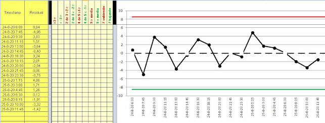
See   SPC Analysis

No out of control alerts appear in this SPC chart of the residuals, so there is no evidence of significant process changes.

Notice that we have a timestamp next to each residual. That would be the timestamp, of the moment each experiment was performed. 

It is essential to collect these timestamps, to investigate any anomalies detected during the analysis.  Timestamp

Conclusions

• Design of Experiments (DOE) is a powerful methodology, for process improvement.

• It enables the identification of critical process factors, based on data, rather than impressions.

• We can estimate the optimal values of these critical factors, to optimize the process.

• Excel provides some useful Data Analysis tools, to achieve this.

• Some processes outputs, don't have a linear relation with the critical factors. In this case we will need a more sophisticated formula such as RSM:   Response Surface DOE with Excel

• Another non-linear example:   The Catapult exercise