Theory of Constraints with Excel Solver

 

The Theory of Constraints is a process improvement methodology that emphasizes the importance of identifying the "system constraint" or bottleneck. By leveraging this constraint, organizations can achieve their financial goals while delivering on-time-in-full to customers, avoiding stock-outs in the supply chain, reducing lead time, etc.

Manufacturing Process Example

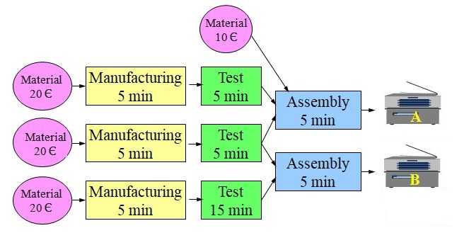
With this simple value stream above, to produce products A and B, we want to illustrate the way to maximize profit taking into account the system constraints.

• Each product is made by assembling two sub assemblies, one of them common to both products.
• The process consists of three sequential operations for which there are special purpose workstations with a corresponding operator each trained for the specific job:
• Manufacturing
• Test
• Assembly
• We want to know how many products A and how many B we should produce to maximize profit.

System Constraints

Product Margin

We want to maximize overall profit so we calculate the margin of each product by subtracting price minus materials cost:

Since we can’t satisfy all the market demand we must decide which product should be our priority. If we ask Finance they will tell us B is the best, since it has the highest margin.

Maximize Product with the Highest Margin: B

Let’s see how many resources we will need to produce all the market demand for B and how many A’s we will be able to produce with the remaining resources:

With the remaining capacity for product A we can:

• manufacture 140 
• only test 40 
• assemble 380 

It makes no sense to manufacture more A’s than we can test. 

The excess assembly capacity will be wasted because we can only assemble the units which have been tested. 

This means that in fact we will only be able to produce 100 B’s and 40 A’s. 

This gives us a total loss per week of 400€.
Maybe the Finance criteria of giving priority to the product with the highest margin was not so good after all.

Bottleneck

We have already noticed that the bottleneck in this line is Test: it is limiting the effective capacity of the whole line.
The use of bottleneck time is, therefore, a critical factor we should consider to optimize the line.
We need to ask ourselves, how much bottleneck time is consumed to obtain a 40€ margin in product A, and the same for product B. 

This means that each minute of test time (bottleneck) if used to test product A gives us a margin of 4€ while product B only gives us 3€.

Product A is, therefore, more profitable in these circumstances.

Maximize Product with Highest Bottleneck Profitability: A

So when we take into consideration the existing constraints A is more profitable. Let’s give priority to A and use the remaining capacity to produce B:

It is, indeed, more profitable to maximize product A in this case in spite of its lower margin.

The bottleneck plays an important role in finding the optimal solution: it defines the effective capacity of the whole line, therefore we need to optimize the use of bottleneck time.

Capacity Utilization

We can clearly see that due to the existing constraints this line is very inefficient. 

Let’s look at the capacity utilization of each operation:

The only operation with 100% utilization is test. This is what we would expect since it is the bottleneck. 

We see that final assembly has very low utilization (less than 50%).
We can see that the only way to improve further the productivity is to reduce test time by making it more efficient or to transfer some work (if possible) to the assembly operation.

Graphical Solution

Let’s now look at the problem graphically:

The red area is the forbidden area due to the constraints: 

• Maximum demand for A
• Maximum demand for B 
• 2400 minutes available at the bottleneck (test): each A consumes 10 minutes of test and each B 20 minutes.

We now look at the point of maximum profit: It will be the furthest point from the origin within the allowed area (green), which is the point of maximum A (200 units) and 20 units of B.

Solution with Solver

Download this Excel file Solver1.xlsx from OneDrive. Open sheet Production 

Now let’s see how to solve the problem using Microsoft Excel Solver. 

First we need to set all the data in a spread sheet:

In matrix B3:D4 we have the unit times for each operation in products A and B.

Column E has material costs and F product selling price. In column G (margin) we have a formula which just subtracts F – E.

In column H (Produced) we want Solver to place the results we are looking for: number of A’s and B’s to produce.

 Column I has the market constraints for A and B.

Row 5 has the formulas above to calculate time consumed on each operation based on the products produced. These values we will compare with row 6 (available times for each operation)

Finally B10 has the shown formula to calculate the profit. This is the cell we will ask Solver to maximize.

Solver Parameters:  

Now we enter Data > Solver to setup the parameters as shown:

We want to maximize Profit (B10)  changing cells H3:H4 where Solver will place the solution we are looking for.

The constraints in Solver:

• B5:D5 ≤ B6:D6       Used times ≤ Available times
• H3:H4 ≤ I3:I4          Don’t produce above market demand
• H3:H4                      Must be integers and not negative

Press resolve and we will get the results:



This confirms the optimal solution we had already found.

Process Improvement

Now imagine that an engineer has found a way to reduce test time of product A from a total of 10 minutes to 9 minutes by adding some work to the assembly operation which would involve an increase from the previous time of 5 minutes to 7.
This suggestion would be difficult to justify with Finance, since we are increasing the overall operator time of product A one minute.
But let us look at our Excel to see what Solver has to say:



We have been able to produce 10 more B’s increasing the profit from 1200€ to 1800€.
This is telling us that maybe the way we compute product profit may not help when we have idle time in some of the operations.

Container Distribution Example

Open sheet Distribution in Solver1.xlsx 

Now let’s see another example of Theory of Constraints solution with Solver:

In this case we want to minimize the cost of distribution of goods containers from warehouses X, Y, Z to shops A, B, C, D, E, F:

Matrix C4:H6 contains the transport costs of one container from each warehouse to each shop.
Matrix C9:H11 (Yellow cells) will contain the number of containers from each warehouse to each shop we are looking for.
The blue cells have the formulas shown.

Constraints:

• Available containers on each warehouse
• Container demand from each shop
• Numbers of containers should be integer (no decimals) and not negative

The Solver parameters will be therefore:

Notice we must meet all the shops requirements: C12:H12 = C13:H13
And the resulting solution from Solver is:

This is the optimal solution which meets all the constraints.

Cargo Plane Loading Example

http://people.brunel.ac.uk/~mastjjb/jeb/or/lpmore.html

A cargo plane has three compartments for storing cargo: front, centre and rear. These compartments have the following limits on both weight and space:

Furthermore, the weight of the cargo in the respective compartments must be the same proportion of that compartment's weight capacity to maintain the balance of the plane. 

The following four cargoes are available for shipment on the next flight:

Any proportion of these cargoes can be accepted. The objective is to determine how much (if any) of each cargo C1, C2, C3 and C4 should be accepted and how to distribute each among the compartments so that the total profit for the flight is maximized. 

We will put all this data in Excel (sheet Cargo):

Constraints:

• Available cargoes 
• Compartment capacities
• Maximum compartment loads
• Compartment load balancing

Solver parameters:

We run Solver to get the optimal solution which meets all constraints:

Conclusions

• All Value Streams are subject to multiple constraints such as:
• Time
• Cost
• Delivery
• Workforce
• Market demand
• The optimal operating point very much depends on the existing system constraints which may vary along time.
• Product cost and profit depend on capacity utilization
• Microsoft Excel Solver is useful to optimize a Value Stream which is subject to multiple constraints.
• Manufacturing lot size minimization is also dependent on existing constraints