Lot Size: A Value Stream Constraint

System constraints are key when it comes to optimizing our value stream. The process bottleneck limits the overall throughput and it determines such things as manufacturing lot sizes.

Learning by doing is an effective way to understand how a value stream works.

With this simple manufacturing line simulation you can experience the effects of alternative solutions in order to maximize profit. 

When resources are shared by several products there is a setup time when changing product and you have to decide what is the optimal production lot size to optimize the process.

Download this Excel file TOCeng5.xlsm from OneDrive folder Polyhedrika

Close other Excel files before you open this one and enable Macros.

Process Objective

Run the simulator to obtain the maximum profit after one simulated week.

You have an initial capital of 1000 € which you can use to buy materials to feed the blue, green and brown machines.

Fixed expenses amount to 2000 €/ week and they will be subtracted from the cash balance at the end of each week.

The market will accept any amount of product P with a unit price of 70 €. Spares P1 and P2 can also be sold but their quantities can never be above the number of products P already sold (if you have already sold 5 P's you can sell, if you want, 5 P1's and 5 P2,s).

Week 1 will start with an empty line so you can simulate one single week leaving an empty line at the end.

You can also simulate several weeks, in which case you don't empty the line at the end.

Manufacturing Lot Size

The green machine performs 3 operations: b, c and d in sequence. All parts should be processed through all 3, so you should decide what manufacturing lot size you want, and process the lot through each of these operations. Before each operation there is a setup time. 

So the sequence is: 

Setup  >  b operation (lot)  >  

Setup  >  c operation (lot)  >

Setup  >  d operation (lot)

In the same way the brown machine has 2 sequential operations: e and f.

 

Simulator Operation

You operate the simulator with these control buttons:

You can either press the start button or use Ctrl + s. The same with the others. The reset button will empty the line and start simulation from zero.

You can halt the simulation at any time to:

• Buy materials (type amount in yellow cells)
• Change operation in the green or brown machines selecting it from the pull down menu (it will start with a setup)
• Transfer Work In Process (Typing amount in the yellow cells)
• Sell finished product or spares (Typing amunt)

This counter will tell you where you are at any time:

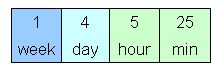
One week has 5 working days of 8 hours. The simulator will stop at the end of each day: Just press start to continue.

Start Simulation

Buy materials for the blue machine, entering the amount in the initial yellow cell.

Buy materials for the green machine, entering the amount in the yellow cell, based on the lot size you have decided.

Then you select the operation you want to run in the green machine from the pull-down menu: b, c or d in this order.

The same with the brown machine: buy materials and select e or f.

You can see these details in the Help sheet:

To transfer to the next machine, or sell,  type the amount on the yellow boxes.

Financial control

You can control your financial situation in real time:

You can buy materials as long as you have enough positive balance.

System Constraints

You may want to try your manufacturing strategy with this simulator before you go into a deeper analysis.

These are the constraints of the different machines:

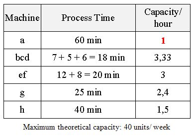
The bottleneck of the whole line is therefore blue machine a: each product P will need 60 minutes of this machine.

You will notice that we are only considering the process times (not the setup times). The reason is that the influence of setup times can be eliminated by using large enough lot sizes as we will see later.

Another constraint is the fact that all products P and spares P1 need machine a (the bottleneck). Spares P2, although they don't need machine a to be produced they can't be sold unless products P (which need machine a) have been sold.

Profitability

The bottleneck (machine a), dictates how much we can produce, and therefore, the profit. We must focus on optimizing the bottleneck time, to maximize profit:

To produce a spare P1, we need 60 minutes of bottleneck time, and we obtain a profit of 30€. 

If we use that time to produce a product P, this allows us to sell also a spare P2 (which doesn't use the bottleneck), and the profit will be 70€.

The conclusion is that we should not produce any spares P1.

Theoretically we should be able to produce and sell 40 P's and 40 P2's per week.

Since we will start with an empty line it will not be possible to achieve this on the first week.

Lot Size

If we decide to produce only P and P2 it will take 60 minutes of bottleneck a to produce one of each. In the green machine we will need to process 2 units: one for P and one for P2; this will take 18 x 2 = 36 minutes of process time.

To process a lot through the green machine we will need 3 setups: one for each operation b, c and d therefore the total setup time for a lot will be = 40 x 3 = 120
If we consider the lot size of the green machine in the time we process this lot size and do 3 setups we need to process 1/2 lot size in the blue machine. 

The process time for the lot size in the green machine is the sum of process times b (7), c (5) and d (6) total: 18. Multiplied by the lot size.

During this time, bottleneck a must process lot size/ 2 units (only for P). If we dedicate all spare time in the green machine to do setups, we conclude that the minimum lot size is 10.

Indeed, to process these 10 parts in the green machine, we will need 300 minutes, which is the time it takes to process 5 parts in machine a.

This means that if we reduce the lot size below 10, the green machine will be more restrictive than the blue, and so it will become the new bottleneck.

In practice, to avoid the green machine from becoming the bottleneck, we must leave a margin, choosing a lot size greater than 10.

If we apply the same reasoning to the brown machine:

In this case the minimum lot size is 8. It may not be practical to have different lot sizes in both machines, so we may decide on a value above both, such as 12, to compensate for any inefficiencies.

Possible Results

Theoretically, starting with a full line, we should be able to produce and sell 40 P,s and 40 P2,s which gives us a weekly margin of 40 x 70 = 2800 €. If we subtract the weekly fixed cost of 2000 € that leaves us a profit of 800 €

Starting with an empty line and leaving it almost empty at the end of one week we obtained the results:

Capacity Utilization

On the top right corner of the simulator, we can keep track of the capacity utilization on each of the machines.

At the end of the week we obtained the following results:

The first thing we notice, is that the bottleneck a has been producing almost 100% of the time: one minute lost in the bottleneck would be a loss for the whole line.

The green and the brown machines, have been stopped at the end of the week, in order to empty the line, and also due to inefficiencies in the manual interventions.

We can see the impact of the setups in these two machines: these consume 30% and 20% of their capacity.

Machines g and h, were stopped at the beginning of the week, due to the empty line, and also along the week due to their excess capacity.

 

Capacity Increase

With this line the maximum capacity we can expect, starting with a full line, is 40 products P and 40 spares P2 per week (one shift).

If we need to produce more, the first step would be to try to reduce the process time in the bottleneck (machine a). If we still don't have enough capacity to cover our customer demand, we may think of duplicating the blue machine.

Bottleneck Capacity Increase

See this analysis in sheet Case 2.

Suppose  we have been able to reduce process time for the blue machine a to 45 minutes (from the previous 60):

We calculate the capacity of each machine and the machines required to produce each product: P, P1 and P2.

The bottleneck is still machine a  (lowest capacity of 1.3)

We want to decide in this situation the combination of P, P1 and P2 which is most profitable:

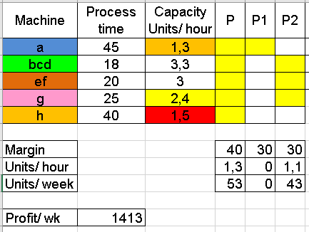
If we produce a P1, we obtain a margin of 30€, but we consume a part from the bottleneck "a", which means, one product P and one spare P2 less (a loss of 70€).

Therefore, we don't want to produce any P1: only produce P and P2.

We use all our a capacity to produce P, so, theoretically, we should be able to produce 

1.3 x 40 = 53 products P per week.

We use the remaining capacity of g (which is the next constraint) to produce P2: 

(2,4 - 1,3) * 40 = 43 spares P2 per week

An increase of the bottleneck a capacity from 1 to 1.3 per hour (30% increase)

has increased our profit from 800€ to 1413€ (77% increase) 

Lot Sizes

We have not considered, so far, the lot sizes. To obtain the previous profit they should be large enough:

We see a significant increase in the minimum lot sizes, due to the fact that the spare time, in the green and brown machines Vs the bottleneck is now lower: there is less time available for setups.

If we use lot sizes lower than those, the machine will become the new bottleneck: more restrictive than the blue machine.

Lead Time

Lead time, from the moment we purchase the materials, until we sell a finished product P, is an important metric of the value stream. In real life, this lead time may require borrowing from a financial institution, and therefore paying interests. 

Operating in lots (in the green and brown machines) has a significant impact in lead time. 

In sheet Leadtime we produce a Gantt chart of the value stream, which in the case of lot size = 10 is:

Total lead time from the moment we purchase the materials until we sell the first product P is 365 minutes.

Now in the case of productivity improvement (a process time = 45 min) Lot sizes need to be higher than 32 and the impact to the lead time will be:

Now the total lead time is 785 (more than double).

In our simulator, this will show in the fact that we will run out of money, before we start to sell product: we will need an initial capital higher than 1000 €. 

Conclusion

• System constraints need to be considered, when it comes to optimizing a value stream
• The bottleneck defines the maximum possible throughput for the total process.
• The bottleneck defines the rate at which product should be started in the line: starting above the bottleneck capacity will only build up Work In Process, and it will not increase throughput.
• When the bottleneck capacity is increased we hit the next bottleneck.
• In machines with several operations, we want the minimum manufacturing lot size, but not so small that it becomes the bottleneck of the total process.
• Capacity utilization should be 100% in the bottleneck, but not necessarily in the rest of the operations.
• Lot size increase, will increase the effective capacity of the machine, but it will also increase the level of WIP in the line, and also the total lead time. 
• Leaving an empty line at the end of the week, to meet weekly production, creates a big problem the next Monday, where most of the line will have no product to work on.