Value Stream Constraints: Variation

Process variation has been described as a virus infecting the value stream: it causes chaos and it is often undetected. Dice Throwing Exercise
A bottleneck limits the effective capacity of the whole line. Bottlenecks caused by variation are more subtle and difficult to detect and act upon. Process simulation can help us experience the effects of different types of constraints, try solutions and detect possible side effects.
Process simulation helps us understand the value stream dynamic behavior: how variation affects key process metrics such as WIP, Lead time, Throughput, Cycle time, On Time Delivery, etc.
Understanding these dynamic effects will enable us to get to the root cause of problems implementing definite solutions and not just containing the symptoms.

Process Flow Concepts
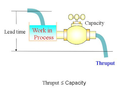
THRUPUT (or THROUGHPUT): Number of items actually processed per unit of time.
CYCLE TIME: Time elapsed between two consecutive outputs.
TAKT TIME: Cycle time required by the customer or market demand.
WIP (Work In Process): Number of items being processed or waiting to be processed.
LEAD TIME: Total time in the system (process plus waiting).
Thruput could be defined for one single workstation or for a whole line. In the case of dealing with a whole line thruput is what comes out from the last workstation.
Work-in-process may be defined again for a single workstation or for the whole line and it includes all the items in the system either being worked on or waiting.
A stable system may be defined as one where the work-in-process and the thruput are stable (in statistical control).
In a stable system with no losses the rate of items entering the line is equal to the rate leaving it.


Thruput = WIP/LT = 4/40 = 0.1 unit/min = 6 unit/hour
In the following chart the curve on the left represents the cumulative number of items started in the line. The curve on the right is the cumulative number of units finished. From hour 0 to 25 the process is stable: the starts line is parallel to the finishes. The horizontal distance between these two lines represents the lead time (time elapsed between one item being started and being finished). The vertical distance between the two lines represents the WIP (number of items in the system in that moment in time).

We assume that each item being started has to wait its turn in a queue until all the items which are already in the system are processed at the thruput rate. The total time in the system for this item will therefore be the time to process all the items in the system including itself.
From hour 25 to 30 we have decided to stop all starts in the line, as a result the WIP has been depleted (from 20 units it has gone down to 10) and therefore we see that lead time has also been halved (from 10 hours to 5 hours).
From hour 30 onward the line is also stable.
The thruput of the line in this chart is the slope of the finish line. its value is 2 items/ hour.
We can see that the slope has remained constant all the time, therefore lead time varies proportionally to WIP:
LEAD TIME = WIP / 2
Additional Flow Concepts
JUST-IN-TIME (JIT): Buffer capacity constraint (stop if output buffer is full)
CAPACITY UTILIZATION: Rate between customer commitment and line capacity
YIELD: Rate between good items and total items processed.
COMPOUND YIELD: Resulting from all step yields.
BATCH MODE: Process items from several periods in one go.
Just-In-Time can be achieved by limiting artificially the output buffer capacity to a minimum in such a way that nobody is allowed to process an item unless he has room for it in the output buffer. This empty space is created when the next workstation removes an item from the buffer. If we follow the same procedure up to the end of the line we see that it is the final customer who activates the whole line by removing finished product/ service from the end of the line. This "hole" created by the customer "bubbles" upstream along the whole line activating as it goes along all the workstations.
This mode of operation is also called a PULL system as opposed to a PUSH system where the items are pushed into the line and they are processed as they come (case of no buffer constraints).
One practical way to implement PULL is Kanban: Kanban Logistics
In some processes not all the items which start in the line find their way to the end: some are lost on the way. This is something common in state-of-the-art technology lines: some items are found defective and non-recoverable and therefore they are discarded along the way.
This effect is also common in business processes: every time there is a control, a signature, etc. there is a possibility of a unit being rejected and therefore not proceeding any further in the process. An example of this is a purchase order which is rejected by the Finance department due to budget restrictions. The immediate consequence of yield loss is that since there are more items starting in the line than items finishing, the capacity requirements in all workstations will not be constant along the line: the first workstations require more capacity than the last.
Batch processing examples:
- Remote process step: items accumulated to fill a lorry
- Reporting at the end of the shift
- Check incident log only once in the shift


Simulator Inputs


Simulator Outputs


Simulator Exercises
1. Ideal Process
You have committed to deliver to your customer exactly 100 items each day. He absolutely needs each one of them. One missing item can cause him a major disruption, therefore if one single item is missing it will be considered as a decommitment. Each item has to be acted upon by 3 different departments in sequence before being delivered to the customer. At the beginning of each day there are 100 items in process on each department and each department is processing 100 items therefore the customer gets at the end of the day the 100 items you have committed. Everything is so perfect that nothing seems to move. If it was not for the clock counting the days at the top right corner of the screen one would think that the simulator has stopped.
SET-UP:


In the ideal case seen before all departments had a capacity to process 100 items per day and that is exactly what they did. In real life this perfect matching of the capacities of the different departments does not happen: there will always be differences in the capacities even if theoretically they ought to be equal. If these capacities are different there will be one department which will have the lowest capacity of the whole line and this department will constitute a bottleneck for the total process. We will call this a "capacity bottleneck" to distinguish it from other possible types of bottlenecks we will see later. The capacity bottleneck may be due to some critical equipment: avon, tester, etc. which is in short supply. The cause may be a critical skill which is in short supply in the organisation. It could be a person who is ill in one of the departments or an authorization which only one person can sign and happens to be very busy.
SET-UP: (Continue from previous exercise)
- Press START to run the simulator
QUESTIONS:
- How is delivery performance? % on time =
- Ave WIP =
- Av Lead time =
- How real do you think this situation is?
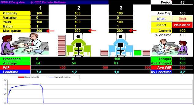
2. Capacity Bottleneck
SET-UP:
- Press Stop to stop simulation
- Change step 2 capacity to 99 (press ENTER )
- Press the Start button
QUESTIONS:

- What happened to delivery performance? % on time =
- Where is the queue building up?
- How is Lead time affected? Av Lead time =
- Why?
- First priority: Customer satisfaction. How can we improve delivery performance if the bottleneck can not be improved?
- How about renegotiating the delivery commitment with the customer?
3. Renegotiate Commitment
In a normal situation it is possible to compensate for a lower capacity in one department by working a bit faster in order to catch up with the work or by working overtime, etc. There are, on the other hand, some cases where there is a physical limitation which can not be compensated by overtime or there are legal constraints, etc. which prevent it. In a case like this, where there is no possibility to open up the bottleneck, all that is left to do is tell the customer and renegotiate with him volumes which are in line with the bottleneck capacity.
SET-UP: (Continue from previous exercise)
- Press the Stop button
- Change Commit to 99 (press ENTER)
- Press the Start button
QUESTIONS:
- How is delivery performance now? % on time =
- Is the queue still growing?
- What is happening to Lead time? Av Lead time =
- Why?
- How can you stop the queue from growing further?
- How about limiting the line starts to the bottleneck capacity?

4. Limit Starts to Bottleneck
The bottleneck is therefore dictating how much you can commit to your customer but it also dictates how many items you should start at the beginning of the line. Starting more than the bottleneck can handle is a waste: the number of units coming out of the line (thruput) will be equal to the bottleneck capacity and therefore all the units started above that capacity will simply pile up in front of the bottleneck increasing not only the inventory but also the lead time.- Change Step 1 Capacity to 99
QUESTIONS:
- Is the queue still growing?
- What about Lead time? Av Lead time =
- Why?
- Why do we still have a queue if the problem has been solved?
- How can you reduce the queue?
- How about limiting starts below delivery level for some time?

5. Limit Starts Further to Reduce WIP
By controlling both the output and input to the line based on the bottleneck capacity we can now say that the problem is solved. But is it really? We see that the lead time is still too long and this is due to the excess inventory which has accumulated in front of the bottleneck. Something similar happens when we have been overeating during holidays: going back to normal eating habits is just not enough if we want to get rid of the extra kilos. In this case therefore you have to flush away the excess inventory and one way can be to limit starts below the thruput level until the excess is depleted.SET-UP (Continue from previous exercise)
- Change step 1 Capacity to 90
- Run (press Start) until the excess inventory is depleted (press Stop)
- Change back step 1 Capacity to 99 (press Start)
OBSERVATIONS
- What happened to Ave WIP when you limited starts below delivery?
- Why?
- What happened to Av Lead time?
- Why?
- Did you miss any deliveries during this operation?
- How can you reduce excess WIP otherwise?
- How about applying Just-In-Time?


6. Apply JIT to Reduce WIP
Another way to eliminate the excess inventory in the line is to apply "Just In Time". This consists basically in banning the accumulation of inventory by decree. The way to do that is to work in "pull" mode: you only produce if there is empty place to put your output. That empty place will only be created the moment the next step in the line removes an item from your output buffer.With this logistics nobody processes more items than the ones going to the customer and in case of excess inventory the corresponding steps stop processing until the excess is depleted. To simulate this method you will fill the line with inventory by putting excess capacity in all workstations for a while. When the line has this excess then it will be depleted applying the JIT method, which is simulated by constraining the buffer capacities to the level committed to the customer.
- Stop simulation
- Reset
- Clear WIP
- Set all Capacities to 500
- Start simulator until line is full (all WIPs = 9899)
- Stop and change all Capacities back to 100

Now we have a balanced line but due to passed problems there is an excess of WIP which causes a large Lead time
- Apply JIT: Set all Max queues to 200
- Start the simulator and watch the effect
Result:

- What happened to the WIP?
- Did you miss any deliveries?
- Is this method of reducing excess WIP safer than the previous one?
7. Variation Bottleneck

Examples of variability bottleneck:
- Test/ quality control step: Test/ Repair Loop
- Public service (mail, transport, customs, etc.)
- Quality problem step
- Sensitive/ critical equipment
- Multiple concurrent input step
SET-UP:
- Stop simulation
- Reset
- Clear WIP
- Set step 2 Variation to 20 (Capacity varies at random between 80 and 120)
- Start simulation
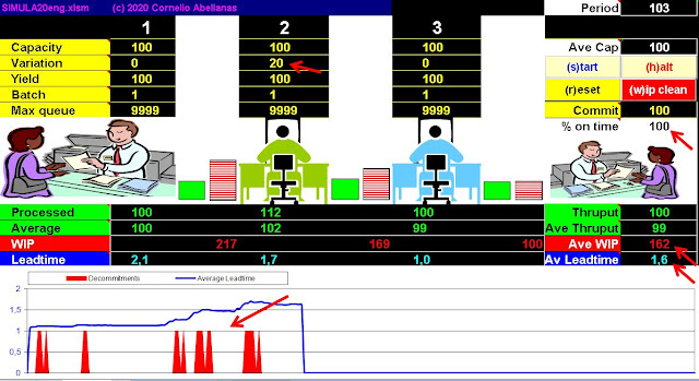
- What happened initially to delivery performance? % on time =
- What is the average production of STEP 2? Average #2 =
- Who is causing the problem in the line?
- Is he likely to admit it? Why?
- Ave WIP =
- Where is the WIP building up?
- Is delivery performance improving as WIP builds up? % on time =
- Why?
- What happened to Av Lead time?
- What can we do to reduce Lead time?
- How about applying Just-In-Time?
8. Apply JIT to reduce Lead time
The purpose of JIT is to reduce excess inventory leaving the absolute minimum required to operate. By doing this waiting time will be reduced and therefore the total lead time will also be reduced. But does it have any side effects?SET-UP: (Continue from previous exercise)
- Set Max queue to 200 in all steps

QUESTIONS:
- % on time =
- What is the average production of all steps? Average =
- Which STEP is causing the problem to the whole line?
- Is it obvious if we just look at the Average line?
- Has Lead time improved by applying JIT? Av Lead time =
- Can Lead time decrease and On-Time-Delivery get worse?
- Would you recommend this solution?
- Why?
- What happens if you have high variability and apply JIT?
- In a case of high variability, how can you reduce lead time and still meet your commitments?
- How about reducing capacity utilization?
Some examples when "Pull" may not be the best solution: https://www.allaboutlean.com/when-not-to-pull/
9. Reduce Capacity Utilization
Assuming we are not able to eliminate the root cause of the problem (variability in STEP 2) how can we meet our customer commitments and at the same time reduce lead time? We will try reducing capacity utilization, which means that we will not commit to our customers 100% of our capacity but only 95%, leaving the 5% balance to compensate for the variability of STEP 2.SET-UP:
- Stop simulation
- Reset
- Clear WIP
- Set step 1 Capacity to 95
- Set step 2 Variation to 20
- Set Commit to 95
- Start simulation
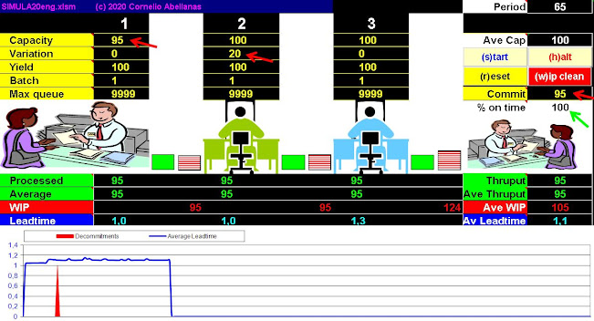
QUESTIONS:
- % on time =
- What are the following values after stability?
- Ave WIP = Av Leadtime =
- What are the negative effects in this case?
- What is the effective thruput in the line? Ave Thruput =
- Would you recommend this solution?

With high variability when capacity utilization approaches 100% then lead time tends to infinity. The reason for this is that variability makes thruput to drop and items start accumulating making the queues, and therefore lead time, longer and longer. With low variability you can get close to 100% utilization and still have a good lead time.
A similar thing happens in a motorway: as soon as the flow of vehicles gets near the motorway capacity speed quickly drops and queues form for several kilometres. This causes the time to increase dramatically.
Point A in the graph represents a situation of high variability and low capacity utilization. If we increase utilization (point B) lead time will increase. If we were able to reduce variability (point C) we would have both: high capacity utilization and low lead time.
Process Yield Loss

Yield loss are items lost during the process. This loss may be due to defects that force to scrap an item or it may be due to the item being rejected in one of the control/ approval steps.
Process Yield Loss Examples:
- Defective silicon wafer scrap
- Scrap after test/ quality control step
- Losses on transport service
- Order cancellation
- Work permit application rejection
In those cases where there is yield loss in several process steps we want to know what the total yield will be in order to size our organization properly.
Examples:
Examples:
- Semiconductor line
- New technology
- Low quality process
A yield bottleneck is typically a control step where rejection of some items may take place
10. Yield Bottleneck
SET-UP:- Stop simulation
- Reset
- Clear WIP
- Set step 2 Yield to 99
- Start simulation

- What is the total thruput in the line? Ave thruput =
- Is lead time affected in this case? Av Leadtime =
- How many units do you start in the line on each period and how many do you finish?
- Average #1 = Ave thruput =
- What happened to the difference between started and finished units in the case of a capacity bottleneck?
- And in this case of a yield bottleneck?
11. Compound Yield
In a process where items are lost/ rejected in several steps we want to know what the total process yield will be as a function of the step yields. This is what we call compound yield.
SET-UP
- Set all step Yields to 90

OBSERVATIONS
- What is the total line yield? Ave thruput =
- Is it what you would expect?
- How do you calculate total yield from step yields?
- Is 90% step yield acceptable?
- What would happen with larger number of steps?
- What happens to the difference between the units started and those delivered?
12. Additional Capacity to Compensate for Yield Loss
How can we estimate the capacity requirements for each process step in a case of yield loss? What are the buffer size requirements? What we want to achieve is deliver the customer requirements with the minimum capacities possible and keeping the minimum amount of inventory to reduce lead time.ASSUMPTION:
- Yield = 90 in all steps
OBJECTIVES:
- Commit = 100
- Av Leadtime = 1
- % on time = 100
- Estimate the minimum capacities required to achieve this:
| 1 | 2 | 3 | |
| Capacity |
- What is the cost of this solution? Ave Cap =
- How can you make lead time equal to 1 while meeting delivery commitments?
- How about limiting the maximum queues?
| 1 | 2 | 3 | |
| Max queue |

Batch Mode Operation
When transportation between two locations is involved you accumulate WIP to fill a van/ lorry and then the whole batch is moved.Batch operation means accumulating items for a number of periods and processing them all in one period. This simulation will assume that the average capacity of the batch-operating step is still the same as in the rest of the steps.
Batch mode examples:
- Daily transport/ delivery
- Fill avon before cooking batch
- Burn-in run with full chamber
13. Batch Mode Effect
A step with a batch period of 5 and average capacity of 100 will process no items during 4 of the periods and 500 items in one single period (the average will be 100 per period).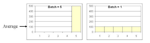
SET-UP:
- Stop simulation
- Reset
- Clear WIP
- Set step 2 Batch to 5
- Start simulation


QUESTIONS:
- Is the batching of STEP 2 affecting the thruput of the total process? Ave thruput =
- Is it affecting on-time delivery? % on time =
- What is the effect in WIP? Ave WIP =
- How is lead time affected? Av Lead time =
- Why?
14. Low Yield + Variability
In real life we will not find single effects as seen so far, but rather a combination of the different effects. When several effects coexist we will not find a single optimal solution. Depending on the relative cost of capacity Vs inventory/ lead time the optimal solution will vary. Typically increasing capacity drastically will solve the problem but it will be an expensive solution.
SET-UP:
PROPOSED SOLUTION:SET-UP:
- Select Simulator tab
- Stop simulation
- Reset
- Clear WIP
- Yield = 99 in all STEPS except #1
- Variation = 10 in all STEPS except #1
- % on time = 100
- Minimum average capacity ( Ave Cap )
- Minimum leadtime ( Av Leadtime )
- Required capacities and Max queues:
1 2 3 Capacity Max queue
- Resulting Ave Cap =
- Resulting Av Leadtime =
- % on time =

15. Bottleneck Effect Recap
The different bottlenecks we experienced produce different effects on the process parameters. Let us recap in order to compare. In real life we will find combinations of a number of these effects and therefore we might need a number of corrective actions in order to improve. Indicate how each parameter will be affected in the long run.
Conclusions
- An instant picture of your Value Stream may not be enough to understand what is going on
- Variation is like a virus which passes undetected unless you are aware and measure it
- Waiting times may be caused by variation in which case you will not be able to reduce them unless you attack the root cause of variation
- Different types of constraints cause different effects which need to be understood in order solve them
- Pushing product through the Value Stream above the bottleneck capacity will only increase WIP and Lead Time but not Thruput
- Applying Just-In-Time to a high variability process is a formula for disaster
Further Value Stream Simulation
- You can see the practical way to apply these concepts to more complex Value Streams in Excel Value Stream Map
- When the Value Stream has to process different products there is a setup time involved when you change product and therefore you need to define your production lot size taking into account the constraints: Lot Size and Constraints
- You also need to optimize the production sequence of the different products: Production Scheduling
- A test/ repair station may become a variability bottleneck: Test/ Repair Loop


Comments
Post a Comment