Excel Value Stream Map

 

Value Stream Maps graphically represent process flow as it is actually performed.

Excel Value Stream Map - YouTube

VSM is typically built following a visit to Gemba (where things are really happening) in order to depict what is really going on (rather than the theoretical process described in standards and procedures).

This approach and VSM concepts are excellently described in "Learning to See" by Mike Rother

To follow the value stream you can follow a product along the manufacturing line or a customer order along the administrative value stream like in   staple yourself to an order

Horizontal Vs Vertical Flow

Value Stream Maps are typically designed to flow horizontally left to right. When a value stream is complex it becomes difficult to view the whole picture: it may require several pages and this makes it difficult to follow..

Making the VSM vertically allows us to visualize complex value stream in a single page.

 

Post-its on Brown Paper

Another common practice is to map the value stream by sticking post-its on a wall or large wrapping paper.

A dedicated room is normally used called Obeya or War Room.

This method has the advantage of simplicity: 

• All participants write post-its in parallel and stick them on the right sequence on the wall.
• Sequence can easily be changed just by moving post-its
• Swim lanes can be drawn to specify who is doing what

Who Does What?: Swim Lanes

Every time there is a change of hands there is an opportunity for waste: waiting time.

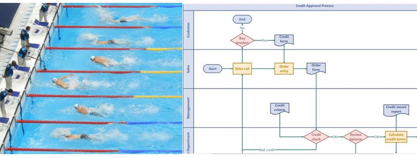
Therefore the VSM should clearly indicate who does what.

Paradigm Shift

"Operators are good at handwriting but many have problems with typing"

I suggest an experiment to see if this paradigm is still valid today:

1. Pick a line operator at random and ask him to type a piece of text in his phone measuring the time it takes
2. Ask the same operator to hand write the same text in a post-it and measure the time
3. Now ask someone else to read both messages

Which was quicker?

Which was easier to read?

The wide use of smartphones today by everyone may have changed this paradigm

Some Limitations of the Post-it Approach

• The Obeya room used to build the VSM is blocked and can't be used for other meetings or activities
• It becomes impractical to save all the work done to continue working on it later on.
• All the hard work done during several hours often ends up in a long roll of brown paper with post-its stored in a cupboard which no one looks at again.
• It is also difficult to communicate to others: photos of hand written post-its are difficult to read.
• Some value streams involve several remote locations so a physical Obeya is not practical
• If you ask other people, not present in the VSM exercise, to give their input they can not view it clearly and propose modifications to the work you have done.

VSM Directly Built in a Spreadsheet in the Cloud (Google Drive or One Drive)

Another alternative to this post-it approach is to build the VSM in a spread sheet with the help of PCs, tablets or smartphones.

  

You can draw your VSM directly using Google Spreadsheets in Google Drive and give write access to your document to all participants in the team and it will take shorter to build the VSM than if you have to write and stick the post-its. You can even have team members participating from remote locations.

People, nowadays,  are quicker and more skilled at typing into their smartphones than hand writing post-its (specially if someone else has to read them). They can easily type while they discuss the VSM with the team.

You can use a Virtual Obeya Room to house the VSM and use, as required, a room with a projector as physical Obeya during the initial VSM construction.

The first step is to go to Gemba: the team has a good look at what is going on and then they gather in a room where the VSM being built is projected on the wall (large screen if possible). All participants write the process step descriptions with their portables or smartphones into the spreadsheet in Google Drive that is visible on the wall. Typing into the spreadsheet can also be done with voice using the smartphone (that's how I do it since I am no good at typing) .

The VSM can also be built directly in the cloud while visiting the line with the smartphones of the participants.

In this group exercise it is easy to make changes in the sequence, insert new steps, etc. At the end of this process we have a workable VSM agreed to by all participants which represents the current state as seen in Gemba.

After the current VSM is concluded we give write access to all process participants including those who were not present in its elaboration, in this way they can make modifications to make sure the VSM reflects what is really going on in Gemba. We might discover that we have more than one process, for instance the night shift is doing it differently. Google Drive keeps track of who has made what modifications.

We also give read only access to the VSM in the cloud to other people and plot an A1 size copy to stick on the department or line wall for everyone to see.

We keep backup copies of the different stages in the modifications to make sure we can go back to a previous version.

I find it very useful to indicate who does what in the VSM instead of making another separate document. In order to do this we include participant swim lanes on the top headers which are easily filled while building the VSM.

In the example above you can notice that the switchboard participates in the process on several occasions.

 

Complex Value Streams

More complex VSMs with feedback loops can be done with Excel such as:

  

Download this Excel simulator VSMandSimulation1.xlsm  from OneDrive 

Share your VSM in the Cloud with Microsoft's Onedrive

In a complex process as the one above Google Drive is not able to manage the graphic flow chart so it is best to use Microsoft's OneDrive:

Excel VSM Advantages:

1. The team involved in the VSM exercise can be located in remote locations and they can all share a spreadsheet in the cloud communicating via Zoom, Meet, Teams, etc.
2. To insure your VSM represents the current reality (hidden factory) rather than a theoretical process flow you need to validate your VSM with all other participants who were not in the room: line operators, suppliers, maintenance, etc. You can not start improving until you are certain of what the current reality is. This is easily done by giving them access to the VSM in the cloud.
3. All the work done is not lost at the end of the meeting and it can be updated remotely at a later stage by all process participants
4. You can easily keep track of the different versions of the VSM as you implement your improvements and you can even go back to a previous version if something goes wrong
5. You can go to Gemba with your VSM on your tablet or smartphone and directly enter process times, WIP, etc. on your VSM in the cloud.
6. Excel allows the addition of the process parameters for each process step by adding as many columns as required on the right:

• Process time
• Setup time
• Cycle time
• Work-In-Process waiting

Complex Process Data Collection

After we all agree with the Value Stream Map we need to collect the data. For a simple process, if no data is available we can manually collect the data in the line. This will give us a rough estimate of process times of each step.

Collecting WIP data manually may not be very useful since the values may vary widely depending on the moment we visit the line.

Process times may also have significant variation.

Process Times Collection: Timestamps  

Ideally we must define data collection points along the process and collect data automatically if possible. If data needs to be collected manually we can use a bar code scanner to read the product serial number on each point and the current  timestamp can, automatically, be collected in the spreadsheet.

 

 

We can analyse these collected data with pivot graphs:

Process Times Collection in Gemba

After we have agreed on the VSM flow (who does what and when) we need to go back to Gemba to collect process times and WIP data for each process step. 

If we use the Excel approach, we can access the VSM we have just produced and directly enter the numbers in our spreadsheet with our smartphones.

It is easy to share this work among all participants each taking care of a few process steps.

They can all write simultaneously into our VSM in the cloud.

We enter average process times in column K and standard deviations in column L

We enter the % of YES data in column N:

Average time to receive a product is 2 min and its standard deviation 1 min.

On average 20% of products received for repair are under warranty.
 

Inter Arrival Time

Average inter arrival cycle is 5 minutes therefore this is the takt required for our complete repair line.

  

Looking at the inter arrival times histogram we notice they follow an exponential distribution, something quite typical while operation times are close to normal distributions.

From this analysis we can enter average inter arrival time in cell K3

Takt Vs Cycle Time

To have a balanced line cycle time of every step should be below takt time (inter arrival cycle) 

  

Average measured repair cycle of 5:31 is a bit larger than the target of 5:02 which is the takt time defined by the average inter arrival time

VSM with Feedback Loops and Alternative Routes

Complex processes require often feedback loops: repair failing items and test them again. These loops are an essential part of the VSM because they often become the bottleneck for the total value stream.

 

  

When the process doesn’t have a single flow but there are several branches you need to estimate the proportion of items that will flow along each branch and this you can do by collecting data along a period of time.

Throughput in the Different Process Steps

Since not all products flow through all steps we need to know the proportion of the throughput entering the line which is flowing through each step. This is reflected in column O

• All products entering the line flow through the first 3 steps (100% in column O). In step 4 (line 6) only the products which are not under warranty are processed: 80%.
• In line 7 only products to be returned to the customer without repair are processed: 4%.
• In the repair step (line 10) 100% of products need to be repaired but some products more than once: those failing Functional or burn-in tests. 119% of products need to be processed.

 

Line Staffing Calculation

We are going to calculate the staffing required (Full Time Equivalent) for each process step in cells M4 to M13 using Solver.

In order to balance the line we need the right staffing on each step to insure enough capacity to handle the product arrivals. This means that Cycle time  ≤  Inter arrival time (takt).

Cycle time = (Average time)  x  (% Throughput )  /  (Staffing)

We calculate the total staff required in the line in cell M1 by adding all the yellow cells in column M. This cell value is what we want to minimize as long as we meet the requirements that all cycle times P4:P13 are below the inter arrival time in K3.

  

We are adding the constraint M4:M13 ≥ 0.1. The proposed staffing by Solver in the yellow cells M4:M13 is shown above.   

Which gives a total staff of 13.3 (M1). This is a theoretical minimum which assumes all staff has all skills, which is not, usually, the case.

Skill Constraints

In cells D1 to H1 we obtain the compound for each process participant (some perform several operations). These values are obtained from those in column M.

If Receive and Coordinator can be combined we may have to round up the sum of the two from the 1.6 requirement to 2.0  

We simulate this by increasing the values in the yellow cells of column M

Invoicing we round up from 1.8 to 2. Test from 2.9 to 3 and repair from 7.4 to 8.

This manual rounding will lead us to this situation:

Where the total staff has increased from the theoretical 13.3 to 15 after considering the different skills required in the different steps.

This increase in the staffing has an effect on lowering the cycle of the steps affected below the takt time of 5 minutes.

Looking at the % Throughput column we notice that some steps only process 4% of the products to be repaired while test and repair have to process 119%. The reason for this is that only 80% pass the test OK the first time. This means 20% have to be tested a second time. Same with burn-in, where 5% fail and have to be retested.

Work In Process and Lead Time

When we visit Gemba to collect process times we can collect also the number of products waiting to be processed before each workstation this is WIP which is in column Q of our chart. Q1 has the total WIP in the line.

 

Every product arriving to a workstation will have to wait in the queue until it is its turn to be processed. Column T has the lead times for each product to be processed on each workstation taking into account the length of the queue. This is calculated with Little's law: 

Lead Time  = WIP  x  Throughput

T1 has the average total lead time (hours) for one product from the time it is received from the customer until it is returned repaired.

Value-Add-Time Vs Non-Value-Add-Time

Column K has the average process times for each operation. 

K1 has the total average process time for a product taking into account that not all products go through every process step as shown in column O. In this case it is 66 minutes.
Just now the total average lead time to repair a product is 15 hours as shown in T1. 

Out of these hours we are only adding value for 66 minutes (total process time), as shown in K1. The rest of the time is waiting time along the different workstations which is non-value-add
The difference 

Lead Time - Process time = 15:00 - 01:06 = 13:54 

is the Non Value Add Time

The ratio VAT / NON-VAT is therefore 

01:06 / 13:54 = 7.9 %

We must bear in mind that the WIP data we have collected from Gemba has typically a lot of variation so this ratio we have calculated may vary widely depending on the moment we visit the line.
This is why we need to collect variation data and use simulation to get a more realistic picture.

Convert your VSM into a Simulator

We will add some additional columns to our VSM converting it into a simulator in: How to convert your VSM into a simulator to experience variation

Conclusions

1. A value stream map allows us to understand who does what and when
2. We should build the map after a visit to Gemba (where things are happening) to make sure it represents the current reality
3. One alternative is to make the VSM directly in a spread sheet in the cloud where all team participants have write access
4. Typing into a smartphone is a common skill nowadays which we can use for data entry into the VSM
5. Both process description and data can be easily typed, or entered with voice, with any smartphone
6. This VSM in the cloud can be easily shared with other process participants in order to validate it
7. After validation all those with a need to know may be given read access to be able to consult it at any time
8. When it comes to implementing improvement actions we can easily keep track of the new versions of the VSM as it evolves
9. Process data collection directly into the VSM can be validated the moment it is entered to avoid data entry errors
10. Analysis of the value stream data can easily be done in the same spreadsheet using Excel Data Analysis tools 
11. To understand the effect of variation in the value stream we can easily convert our VSM into a simulator.