Response Surface Design Of Experiments with Excel

Design of Experiments is a useful methodology for process improvement. The purpose is to find a relationship between process variables we can control and key process outputs in order to increase process capability.

You can use Excel statistical analysis tools, Solver, Pivot charts, etc. to plan and analyse the results of these experiments.

The first approach is to look for a linear relationship as shown in:  Excel DOE

But in some cases this relationship may not be linear, in which case we will try a quadratic model with Response Surface DOE.

We will use an example in this Excel file you can download:

Download file  ExcelResponseSurface.xlsm  from OneDrive to your PC.

In this example we are trying to maximize process yield acting on the critical factors pH, Temperature and Time.

We will run the experiments in the Experiments simulation sheet using coded values.

 

Code	pH	Temperature	Time
-1	2	120	7
1	12	150	15

Factorial Experiments

We start by running a full factorial experiment with 2 central points:

We now compute the 2 way interactions by multiplying the corresponding columns in sheet Factorial analysis:

We now use Excel Data Analysis/ Regression: 

This is a confirmation that this linear mathematical model is not valid: R^2 adjusted is very low and all p values for all factors and interactions are above 0.05.

We suspect curvature so we look to the average yield values for the pH inputs with a Pivot Chart:

We can, clearly, see the lack of linearity: Yield for pH = 0 is totally out of line with the -1 and +1 values.

Response Surface Designs

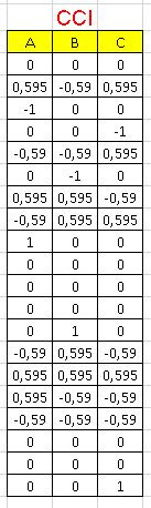
In order to approximate a quadratic model we need two additional values for each factor. In our case of 3 factors we have 2 possible designs as shown in sheet RSMdesigns:



Both CCD and CCI designs involve the same number of experiments (20) but in the case of CCD the two additional values go beyond the values of 1 and -1 we originally wanted to experiment.

In the following table we can see the correspondence between coded and uncoded values for each factor:

We can use the last row of this table to convert any coded value entered in cell J20 to the uncoded values for each of the factors.

We can not run CCD because the resulting pH values are physically impossible (pH varies between 0 and 14)

Therefore we will run a CCI design for 3 factors:

Run Response Surface CCI Experiments

To run the experiments we will need to convert all the coded values in the CCI table to uncoded as shown in sheet Run experiments:

In order to randomize the order in which to run the experiments use a macro pressing Ctrl + o and then follow the order indicated in column I:

To Run These Experiments with our Simulator

In our case we will simulate the experiments by loading the coded CCI design table in sheet Experiments simulation and we will obtain the resulting Yields:

Analysis with Solver

We are going to use two alternative methods for the approximation of a quadratic formula to our data: 

• Solver 
• Regression.

We start with the Solver alternative.

Open sheet ResponseSolver:

The purpose of the analysis is to find a quadratic mathematical formula to approximate the behavior of our process.

This formula will have as terms:

• An intercept coefficient (1)
• Factors each with a coefficient (3)
• 2 way interactions with their coefficients (3)
• Squares of each factor with their coefficients (3)

as shown from J2 to R2.

To use Solver we start by defining where we want Solver to store our results (the coefficients): they will be the yellow cells I3 to R3.

Assuming we already have the results we estimate yield (YieldC) for each experiment in column F with a formula in F3 which we will replicate all the way down. In this formula we use the corresponding factor values in columns B C and D with the coefficients in I3 to R3:

In column G we enter      =(actual yield - estimated yield) ^ 2

In G23 we enter the formula to sum the G column   =SUM(G3:G22).

Now we ask Solver to calculate the values from I3 to R3 to make the total error in G23 a minimum.

 

Then we obtain the coefficients we were looking for in I3 to R3.

Our resulting formula to estimate yield is:

Yield = 20 +15 pH + 0,9 Temp + 6,7 Time - 25 pH * pH + pH * Temp -12,2 pH *Time - 0,1 Temp * Temp -1,5 Temp * Time - 9,1 Time * Time

Process Optimization with Solver

Now that we have the formula to estimate Yield from pH, Temperature and Time we want to find the values that will give the maximum process yield:

We will again use Solver this time to find these optimal values. 

Now we will use the coefficients in I3:R3 we just calculated and the values in I13 to R13. The only values we are asking Solver to calculate are the three factors in J13 to L13. All the other values for interactions and squares are calculated from these with a formula in the corresponding cell. In I13 we put 1 that will be multiplied by the independent term in I3.

In K15 we put the formula for yield which is just the SUMPRODUCT of the coefficients in I3:R3 and the values in I13:R13:

We ask Solver the maximize Yield (K15) with the values of our 3 factors in J13:L13. With the constraints that they should be between -1 and +1.

We obtain the optimal coded values of pH = 0.3, Temperature = 1 and Time = 0.08 and this will give us a Yield = 23.8

Analysis with Regression

Another Excel alternative is to approximate the quadratic formula using regression.

In order to do this we need to build the table of interactions and squares just by multiplying the corresponding columns of the factors as seen in sheet ResponseRegression:

 

We can now go to Analysis/ Regression:

and get the results:

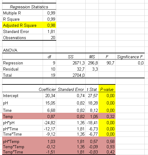
Now we can see excellent R^2 values (0.98) and see which factors and interactions are significant (p < 0.05).

We notice that Temperature and all its interactions have no significant effects on yield (p > 0.05)

Removing these non significant terms We obtain the coefficients similar to those we calculated with solver.

We have a more simplified formula because Temperature was not significant:

Yield = 20.31 + 15.05 pH + 6.68 Time - 24.81 pH^2 -12.17 pH * Time - 9.11 Time^2

This formula is for coded factor values.

Optimize Process Yield with Solver

We can again use Solver to maximize yield:

• We add cells R16 to R24 to house the values calculated by Solver.
• Solver only needs to calculate pH (R18) and Time (R19). 
• R21 to R23 are calculated with a formula from these two values. 
• R17 = 1 to multiply with the intercept coefficient in N17.
• The formula for Yield in R24 is   =SUMPRODUCT(N17:N23;R17:R23).
• The result from Solver is:

We have obtained a similar value for maximum yield.

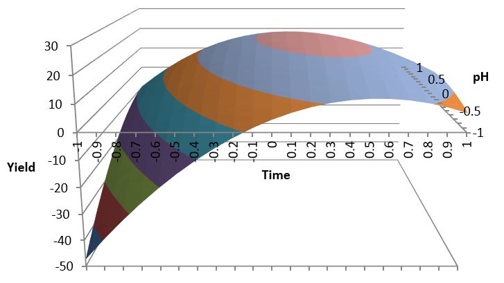
Response Surface Graph

Let's have a look at the shape of this formula:



Now we can understand why the linear model was unable to find the optimal yield: we were trying to represent this with a flat surface experimenting only with +1 and -1.

The red area is where we have the maximum yield and we can confirm the pH and Time to obtain it.  

Another way to see it:

Residuals Analysis

We are assuming that this mathematical formula represents our process but there are some additional checks we should do to validate our assumptions.

In order to do this we are going to analyse the differences between the actual results of our experiments and the estimated values using our formula in sheet Residuals:

Comparing the residuals with the estimated values we should not detect any trends.

Residuals Normality

We expect the residuals to follow a normal (Gaussian) distribution with an average of zero:

The test for normality gives us a p = 0.61 > 0.05 so it is OK (no evidence of lack of normality)

Test for Trends in the Residuals

No trends have been detected along the time the experiments were run (see the timestamps of each experiment)

Confirmation Runs

Now we run confirmation runs with our calculated optimal values for pH and Time and we obtain an average yield of 22.2 with a confidence interval 21.0 - 23.3

Conclusions

• Design of Experiments can be used to approximate linear or quadratic models to our process response in order to understand its behavior.
• It allows the identification of critical factors affecting the response.
• With a regression analysis, we obtain a mathematical formula, to estimate the process response as a function of these factors. 
• We can then find the values of these factors that optimize the response.
• Very often we find a close to linear relationship between factors and response in our area of interest, then we can use a linear regression DOE
• If these relationships are not linear we can use Response Surface DOE as we have just seen.
• All this analysis can be performed with Excel Statistical Analysis tools, Solver, Pivot Charts, etc.
• Another example of non linear DOE: The Catapult exercise