Six Sigma Virtual Catapult with Excel

A wooden catapult has been widely used in Six Sigma education to illustrate multiple factor process variation and optimization.
We will use a catapult simulator with 4 factors to practice:
- Process variation
- Linear regression
- Response surface analysis
- Process optimization

Download this Excel simulator Catapult.xlsx from Google Drive and run it in your PC.

Working Plan
Possible Factors Affecting Range
We have 4 factors that might affect distance d:
f: spring force
m: payload weight
a: release angle
l: lever length
Experimentation Levels

Factorial Experiment Design
First we want to know which of these factors affect the range d.
We will start with a full factorial design with the 4 factors adding 4 central points.
See article Design of Experiments (DOE) with Excel
In sheet Coding we obtain the uncoded values from the coded design matrix.

Run the Experiments

Factorial Analysis


Curvature
The R square value of 0.68 indicates that this linear mathematical model only explains 68% of the variation.
On the other hand the p-values of the four factors below 0.05 indicate that they all have a significant effect on the distance d.

Response Surface Design

To the 16 full factorial experiments already performed we now add 8 additional star points and 7 central points to complete the response surface experiments.
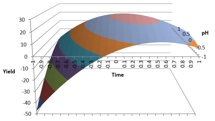
Response Surface Analysis
We now compute the squares and interactions of factors for the analysis in sheet Response:

We do the regression analysis using d as an output and all factors, interactions and squares as inputs.
The result of the regression analysis in sheet Response:

We now have a good R square value of 91%
We will now remove non-significant squares and interactions (p > 0.05) and run the regression again in sheet Reduced:

Maximum Range
We will prepare the cells for Solver to calculate the optimal factor values to achieve maximum distance in sheet Reduced.
We prepare the yellow cells to contain the values of f, m, a, l that Solver will calculate to maximize distance d (R26).
Squares and interactions in column R are calculated with formulas from the yellow cells.
The formula for distance in R26 is = SUMPRODUCT(M17:M25 ; R17:R25):


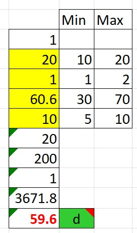
f = 20 (maximum force)
m = 1 (minimum payload)
a = 60.6 degrees release angle
l = 10 (maximum lever length)
Results Confirmation
We run 10 experiments all with these optimal values in sheet Confirmation:


We confirm the maximum distance with an angle of 60º.
Hit Target 20
We now want to calculate the factor values to hit a specific target.
There are many combinations of f, m and l values that will allow us to achieve the target of 20 by changing the angle a.
In sheet Target 20:
We fix f = 10, m = 2 and l = 10 and use Solver to calculate the angle a to hit the target d = 20

The resulting angle is a = 51.2
Average Confidence Interval

Conclusions
- The Six Sigma Catapult is a useful device to experiment process variation, Design of Experiments and multiple factor process optimization.
- Process simulation could be a useful alternative, when it is not possible to use an actual catapult.
- The catapult may be simulated with Excel.
- Group work and discussion is still possible remotely, discussing with a video call.
- Design of factorial experiments, and Response Surface analysis, may be done with Excel Data Analysis.
- Excel Solver may be used to optimize the mathematical model with constraints.
Related Articles
- Another teaching simulator to understand variation: Dice Throwing Exercise
- Design of Experiments (DOE) with Excel
- Response Surface DOE with Excel

Comments
Post a Comment