In sheet
Diameter in column A we have 500 measurements of a critical diameter.
After being confident that our process is stable we can characterize it with descriptive statistics in Excel Data Analysis:

These are the results: basic statistics of our data

Process Stability: Statistical Process Control
All these statistics are meaningless unless our process is stable over time. This we can check with a Statistical Process Control (SPC) analysis. (sheet SPC Diameter):
We see no out-of-control symptoms, so we conclude this is a stable process.
We can, then, assume that our statistical results of this sample, can be applied to our population.
Frequency Distribution Histogram
The histogram gives a graphical representation of this variable.
In Excel Data Analysis we select Histogram. (Sheet Frequency Distribution):

Result:

We see a bell shaped distribution typical of a
normal (Gaussian) distribution. We see that it is quite symmetrical and its mean, median and mode are very similar. This is a very common distribution in nature and many process metrics.
Test for Normality
We want to know to what extent is our
diameter distribution normal (Gaussian). We do this
normality test in sheet
BasicStats diameter:

We can confirm this diameter data follows a normal distribution (p value 0.466 > alpha 0.05)
Meeting this normality condition is a prerequisite for the validity of our SPC test we have just performed .
Process Lead Time
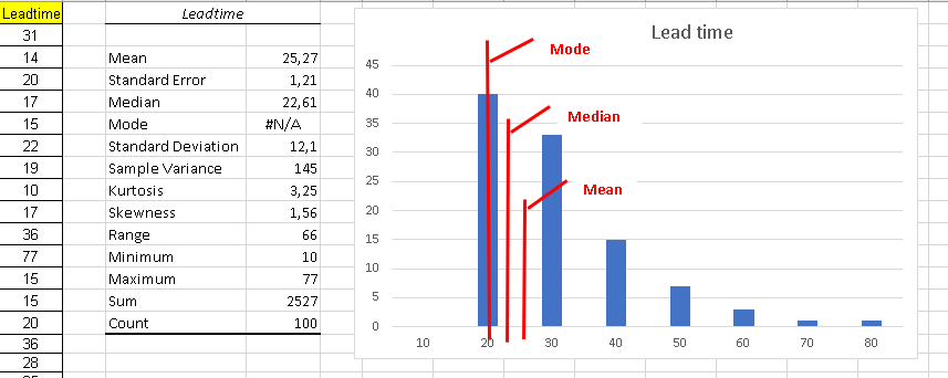
In sheet Lead time We have collected process lead time (hours).
We do the same analysis:
In this case we see a very skewed distribution
We also notice that Mode, Mean and Median are quite different from each other.
Let us check now manufacturing lead time normality (Sheet Basic Stats Leadtime):
In this case the distribution is very skewed. So lack of normality is confirmed: p = 0 < 0.05
This is something common in time measurements. The reason for the skewness of time distributions is that:
- there is always a physical limitation which makes it impossible for a time metric to be below a certain limit. In this example this limit may be around 8 hours.
- there is no upper limit: things may go wrong and time can become very large.
Customer Requirements
All processes have a customer: either the final, external, customer or an internal customer.
In our process metrics we need to know, not only the nominal value required by the customer but also the spec limits.
For a mathematician the nominal value may be enough, but in real life we know it is impossible to exactly meet any real value: there is always an error (even if it is just a few microns).
The spec limits indicate where the customer starts having real problems, when using our product.
Customer specifications are still necessary in the times of Six Sigma but their interpretation has changed:
In football as long as the ball enters the goal it counts.
In the new approach being within specs is not enough: you better keep away from the limits or else you have a chance of falling over.
Today meeting the customer specifications is not enough: we must prove to our customer that our process is very unlikely to produce a single part outside the specs.
We use the process capability metrics to estimate to what extent is our process able to systematically satisfy the customer (meet the specs).
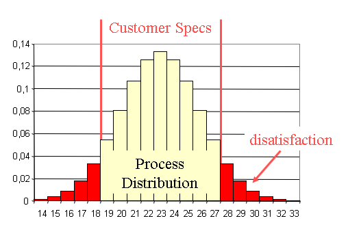
Imagine you measure a critical dimension of the parts you just received from your supplier, and they are all within your spec limit following this distribution
In the old times you would just accept these parts, since they all meet the specs. But those parts close to the spec limit will probably cause you problems. Also:
Looking at the strange shape of the distribution, you can guess that your supplier is producing bad parts, and then removing them before sending them to you.
This is a waste that you will, eventually, end up paying for.
Also the selection used to separate the good from the bad will have escapes so you will. also, receive some faulty parts.
Process Capability
Assuming our process is stable the histogram characterizes the process behavior. We need to compare this with the customer requirements represented by the spec limits.
Process Capability Index Cp
This index is an estimation of the ability of a process to satisfy its customer.
The process capability index Cp is the rate between the spec range specified by the customer spec limits, and our process variation measured by six times its standard deviation:
Cp = (USL -LSL) / (6 σ)
Process Capability Index Cpk
Index Cp is not enough to warrant meeting the specs. If the average of our distribution is not in the center of the spec range we may be out of spec in spite of our narrow distribution.
So we need another index which takes into account the centering of the distribution: Cpk
When the distribution is centered in the spec range Cp = Cpk. If not Cpk < Cp.
- Centering the distribution can, sometimes, be achieved by an adjustment. This will improve Cpk making it closer to Cp.
- Improving Cp implies reducing the standard deviation which is typically much more difficult.
Single-sided Specifications
In both these cases of one-sided specs, you can only use Cpk.
Cp makes no sense since you have no spec range.
This Cpk value below 1 is clearly unacceptable.
Common Mistakes with Capability Indices

Diameter Example Capability
In the previous diameter example we concluded:
- Mean = 99.81
- Standard deviation = 9.77
- Sample size = 500
- Normal distribution (p = 0.466)
If the customer spec limits are:
Before we calculate Cp and Cpk we need to ensure that the process is stable. We will use an Individuals Variables SPC Chart in sheet SPC ind:

We see no out-of-control symptoms so the process is stable.
Now that we know the process is stable and follows a normal distribution we can go ahead and calculate Cp and Cpk:
Cp = (USL -LSL) / (6 σ) = (110 - 95) / (6 * 9.77) = 0.25
To calculate Cpk we look for the nearest spec limit to the mean: LSL = 95
Cpk = (Mean - LSL) / (3 σ) = (99.81 - 95) / (3 * 9.77) = 0.16
We notice that both Cp and Cpk are totally unacceptable.
A Six Sigma process is one with Cpk > 1.5
In a case like this the first step must be to center the process in the spec range:
Make the mean = (110 + 95)/ 2 = 102.5
And the next step would be to reduce the standard deviation (more difficult)
Lead time Capability
In our previous analysis we concluded:
- Mean = 25.27
- Standard deviation = 12.05
- Sample size = 100
- Distribution not normal
In this case we want lead time to be less than 50 hours so we only have an upper spec limit:
The prerequisite of normality is not met so we can't calculate Cp and Cpk.
The solution is to transform the data. We will try a Box-Cox transformation.
We copy the data to the BoxCox sheet:
Now we use Solver to calculate the Lambda value in cell I8 to maximize cell I6.
The resulting lambda value is -0.348 and in column F we already have the transformed data.
We will now check that this transformed data follows a normal distribution by copying it to the BasicStats transformed sheet:
We have, indeed, achieved normality (p = 0.717 > 0.05)
We now check for process stability with the transformed data in SPC transformed sheet:
The process is stable: no out-of-control alerts.
To calculate Cp and Cpk we need to transform the USL of 50 hours.
We must notice that as time increases the transformed values decrease so the Upper Spec Limit will be transformed into a Lower Spec Limit:
Transformed LSL = 50 ^ (-0.348) = 0.256
We get the mean 0.34 of the transformed data from BasicStats transformed sheet:
When we have just one spec limit Cp makes no sense.
We can just calculate Cpk:
Cpk = (0.34 - 0.256) / (3 * 0.05) = 0.56
To find out % late:
=NORMDIST (0,256 ; 0,34 ; 0,05 ;1) = 4.7 % late
Cpk and Ppk
In industry apart from these indices they use another two:
Pp and Ppk.
In this case what we have been calculating using the standard deviation of all the data (sigma overall) they call Pp and Ppk.
And what they call
Cp and Cpk are calculated from an
estimate of the
standard deviation derived from the average range in an
Xbar & R chart.
This calculation requires making several measurements (typically 5) on each instance instead of just one measurement used so far.
The Xbar chart is made with means of each set of 5 values. The Range chart is made calculating the ranges of the 5 values (maximum - minimum).
With this way of calculating these indices, only intrinsic variability is included in the sigma estimate so this gives a lower value for this sigma estimate and therefore higher values for the indices.
This is an example to illustrate these calculations:
The sigma estimate 0.18 is lower than the overall sigma 0.23 so the computed Cp and Cpk are higher than Pp and Ppk.
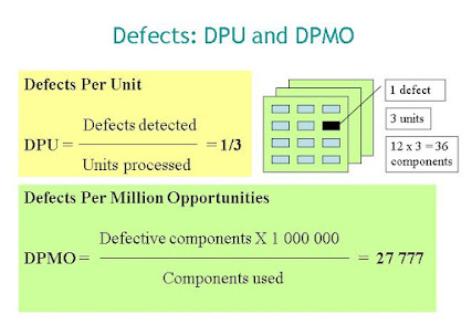
Attribute Process Capability
So far we have been dealing with variables, but sometimes we only have attributes such as Pass/ Fail or Defects per Unit.
Variables can be converted to attributes: for instance we can count the number of items out of spec.
Going back to the diameter example above we can compute the % of parts above the USL and below the LSL.
- Mean = 99.81
- Standard deviation = 9.77
- Normal distribution (p = 0.466)
- USL = 110
- LSL = 95
Since the distribution is normal we can compute the proportion of parts below the LSL:


Comments
Post a Comment