Production Scheduling

 

When we need to process different products in the same line we want to work out the best job sequence to minimize lead time and maximize capacity utilization.

We also need to work out the minimum lot size to meet the demand and minimize lead time.

Before we can commit the delivery date of a new job to the customer we need to know the  state of the jobs already being processed

For non repetitive processes you can use project management scheduling

The ideal of "Lean Production" is lot size of 1 but this is not always possible when change-over time is significant. This change-over involves loading different components and changing jigs or molds. When change over or setup time is significantly higher than process time we are forced to work with larger lot sizes.

One way to minimize lot size is to minimize setup time. The SMED (Single Minute Exchange of Dies) methodology has been very successful to reduce setup times from hours to minutes. 

Scheduling Constraints

In a sequential line products are processed through a number of workstations following a certain sequence but process parameters are typically different for each product type. Each workstation, in order to do the work needs:

• Equipment available
• Operator ready
• WIP (Work In Process) from the previous workstation available

If any of these are missing the workstation stops.

Any of these stops affects all subsequent operations and the overall lead time as seen by the customer. 

We also want to do the job with minimum:

• Equipment time
• Operator time
• WIP waiting

The problem is that unless everything is perfect someone has to wait:

• In the case of a spaceship in order to minimize the astronaut time: a huge team of ground support personnel is available just in case.
• In an airport, in order to maximize the runway utilization (airport bottleneck): planes, pilots, personnel, customers are waiting for take off.
• In Formula I races a 7 second service time is achieved with a team of 10 people doing nothing most of the time during the race and just working very fast and synchronized during those 7 seconds.

In our sequential line in a workstation either the equipment or the operator will be idle or there will be excess WIP.

If WIP waits don´t forget it is the customer order that is waiting.

Case 1: Equal Operation Process Times:

The process is perfect: nobody waits. While WS A is processing Order 2 WS B is processing Order 1 and the total lead time for each order is 4h.

Case 2: Different Operation Process Times

Order 2 will have to wait for operation B to finish with order 1 and therefore Order 2 will take 4h instead of 3 to complete and this will affect the total lead time seen by the customer waiting for this order. Also it will increase the amount of WIP in the line.

The second operation (B) takes longer than the first (A) so it becomes the bottleneck causing an accumulation of WIP in front of it.

Case 3: Bottleneck in Front

Workstation B will be idle until order 2 arrives and this will decrease B capacity utilization.

The lead time seen by the customer (3h) is not affected but we are underutilizing our resources (B)

So Why do we Need Scheduling?

Excel Scheduler

You can download an Excel scheduler for 4 sequential operations:
Download this Excel file  SCHEDULE5eng.xlsx  from OneDrive 



It is used to schedule an electronic circuit assembly line with 4 operations in this sequence:

• SMT: Surface Mount Technology automatic component placement and reflow soldering
• INS: Manual pin-thru-hole component insertion and wave soldering
• ICT: In-Circuit-Test
• FUN: Functional Test

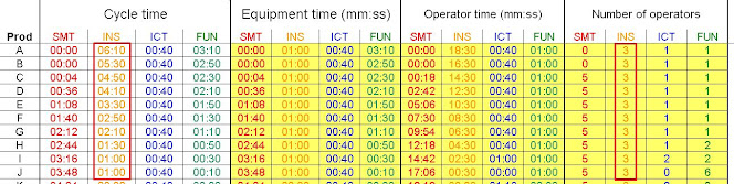
Process Parameters

In sheet Times we must input Equipment times, Operator times and Number of operators for each of the 4 operations and for each product.

Cycle Times are calculated from these: 

 Cycle Time = max( Equipment time ; Operator Time/ Number of Operators)

In this example we want to maximize production with the existing equipment by adding as many operators as required to do this. Therefore:

Number of operators = Operator time / Equipment time (rounding up)

For instance number of operators for Prod A  operation INS = 18:30 / 01:00 = 19 (rounded up)

The scheduler will use these calculated cycle times: 

Job operation time = Setup time + Cycle time  x  Quantity

Setup times for each operation are input in the Main sheet and are assumed to be the same for all products.

With the current number of operators you can notice that Cycle times are identical to equipment times: by adding enough operators we have insured that the line capacity is limited by equipment times and not operator times.

Obviously the number of operators calculated may not be feasible, in which case we enter the available operators and processing will take longer as we will experience later.

 

Main Sheet

• Ord: order in which we want to run the jobs. It should have numbers 1 to 10 in the order we decide.
• Prod: has the products to be produced selected for the ones we defined in sheet Times.
• OK: number of operations already completed (0 to 4)
• Qty: quantities we need to produce of each product
• starting time stamp: day and time we will start producing

Gantt Chart

The Gantt chart shows the scheduling result:



By placing the cursor on the chart we can see the starting or ending time stamp for any operation and product.
WIP waiting times are in light colors and these are what we want to minimize to reduce lead times.
We can also notice when workstations are idle.
In this case, if we start on 6/2/2019 at 6:00 and all 10 jobs will be finished before 12/2/2019.

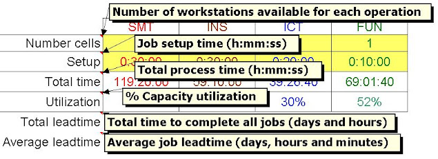
Additional Inputs and Results

• The number of work cells in each operation is 1 by default but we may have up to 5.
• Setup times need to be defined for each operation. In this example it is the time it takes to unload all component reels and load the new ones for the next product. In the case of test it is the time it takes to change the test jigs and load the new program. We assume all products have the same setup times.

The next 2 lines are outputs:

• Total process times of each workstation (no waiting times included)
• Capacity utilization of each workstation. You can notice that SMT with 100% utilization is, in this case, the bottleneck for the whole line.

Total lead time and average lead time are outputs that will affect the customers which we want to minimize.

Schedule for Each Workstation

A detailed schedule is automatically generated for each workstation with starting and ending timestamps and number of operators required.

The actual times can be added on the right columns to be used on the next reschedule.

Bottleneck Scheduling

Looking at the capacity utilization of the 4 workstations we notice that SMT has 100% utilization but all the rest are well below.

This indicates that the bottleneck of this line with these required quantities is SMT. In this case the bottleneck happens to be the first workstation so the following stations are starved of products so they can't process as much as they could: they will be idle some of the time.

The order in which we have scheduled the 10 jobs has been from lowest use of SMT (bottleneck) time to highest use.

Let's see what would happen if we reverse the order: Highest use of bottleneck first:



We notice that the total lead time has increased from 5 days 17h to 7 days: an increase of 1 day and 7 hours.

Average job lead time has also increased from 1d 10h 24m to 1d 13h 16m

Capacity utilizations continue to be very low. 

It is obvious that it makes no sense to schedule products A and B at the end since they do no use the bottleneck so if we just put them first keeping the rest of the sequence as it is we would get a total lead time of 6 days 11h: still worse than the first option.

The first conclusion is that we should schedule focusing on the bottleneck workstation and process from least to most bottleneck use.

 

Bottleneck in the last operation

Let us now keep the same sequence of products but change the quantities to the inverse order:

In this case we notice that this sequence has a lot of waiting time before the INS and FUN operations. Capacity utilization is very good but average lead time is very high: all jobs except the first have a lot of waiting and these long lead times will be unacceptable to the customer.

The bottleneck in this case is FUN: total time for all jobs is 114h 51m 40s much higher than the other workstations.

We notice that with this sequence we are scheduling from highest bottleneck (FUN) use to lowest, so let's try the reverse order:

Total lead time has increased 1d 4h but average lead time has decreased from 3 days 16h to 1 day 10h (less than half).

This, therefore, reinforces our previous conclusion: schedule from less bottleneck use to more.

Schedule with Operator Constraints

Let us go back to the original setup:  

In the examples so far we have assumed that there are enough operators in each workstation so that the equipment never stops but this assumption may not be feasible.

Looking at the schedule for the INSERT operation we are using 19 operators for product A and the number decreases down to 1 for product J.

Let's assume that we only have 3 operators available to perform this operation for all products:



In the Times sheet we enter 3 in the number of operators for all products and the result is that now cycle times have increased above equipment times. This means that now the operators will be the constraint rather than the equipment in the INS workstation.

The resulting schedule is:



Now INS has become the bottleneck and there is an accumulation of products waiting to be processed in this workstation causing waiting time in all jobs. Average lead time has increased from 1 day 10h to 2 days 21h (it has doubled). Total lead time has only increased 10 hours.

 

Cell duplication

Let us now set back the original number of operators for INS: 

In a line we will always have a bottleneck which limits the capacity of the whole line. In some cases we might be able to duplicate the bottleneck workstation to increase the overall line capacity.

Let's duplicate the SMT workstation which was the bottleneck in our first example to see the effect:



Total lead time has been reduced from 5 days 17h to 3 days 15h (more than 2 day reduction)

Average lead time has increased 4 hours: we have waiting in INS and FUN.

We notice that SMT capacity utilization has decreased from 100% to 86% while utilization in the other 3 workstations has increased.

Let's see if duplicate INS and FUN as well:



We notice that total lead time has not improved but average lead time has decreased 9 hours: practically no waiting time.

Since we have increased all capacities capacity utilizations have decreased.

Reschedule

A production schedule needs to be kept up to date at all times in order to be useful. 

All those involved need an easy access to an up to date schedule.

In order to do this operators need to confirm in the scheduler when each operation is completed.

One way to achieve this is to have the scheduler in the cloud (Intranet, Google Drive, One Drive, etc.) and give write or read access to those required. This can even be done with a standard smartphone. 

Let us see how to update our schedule daily.  

Going back to our first schedule starting on 6/2/2019 we normally have to update this schedule at least daily or when a major change has taken place. 

We need to remove what has already been done and add any new jobs. Let's see how do we reschedule on the next day 7/2/2019:



We change our starting timestamp to 07/02/19 06:00 and then input in the OK column: Products A and B completed (4 operations finished) C and D only FUN is missing (3 completed), etc.

If there are any new jobs we would add them at the end shifting all jobs up.

Manufacturing Lot Size

A critical decision in manufacturing scheduling is the manufacturing lot size.

One alternative is to make it equal to the customer order lot size.

The customer may decide to place large orders in order to benefit of lower price offers but this may block the line for long periods affecting other customers. 

One alternative is to agree on breaking down a large order into smaller daily or weekly deliveries to avoid WIP accumulation both in our line and in the customer. 

See how to calculate the minimum manufacturing lot size in Lot Size and Constraints

 

Job Splitting

Due to the setup times every time we change product we may think that the larger the lot size the better. Let's see this effect with a new example:

We need to produce these 5 products with quantities of 500 each.



 What would be the effect of splitting the jobs of 500 into two of 250?



In spite of duplicating setup times we see average lead times have been halved and total lead time is also reduced.

We would, of course, need to agree with the customers to split the deliveries in two

Conclusions

• In order to commit a delivery time to a customer we need to schedule production taking into account existing jobs already in process
• When a job is given priority we need to know the impact to all other current jobs
• Job scheduling enables lead time reduction while increasing resource utilization and therefore effective line capacity improvement
• To optimize scheduling we should focus on the bottleneck
• Schedule jobs from lowest to highest bottleneck utilization
• After total lead time is minimized small changes in sequence will allow the reduction of waiting times and therefore the reduction of specific job lead times.
• By meeting the resulting schedule on each workstation we will insure on-time delivery to the customer.
• Regular rescheduling is required to adapt to the real current situation
• The scheduler could be an essential component of a virtual Obeya Room to keep all involved up to date
• Normally we need to schedule just a few new jobs each day but taking into account all other jobs already in progress
• There is multiple job scheduling software in the market