Multiple Response Optimization with Design of Experiments (DOE)

Design of experiments, is a systematic experimentation, with a process critical factors, in order to correlate these factors to process responses.
In DOE with Excel we obtained a linear relationship, between several factors and one response.
In Response Surface DOE this was extended to non-linear relations.
In both cases we were optimizing one single response. Now we will analyse some cases where more than one response needs to be optimized.

Problem Description
Download file Multiple Response.xlsm from OneDrive to your PC.
We want to maximize yield and minimize cost in a process where we have identified three critical factors which may affect both.
These are the factors and levels we want to experiment with:

Full Factorial DOE
We start with a full factorial with two central points DOE and run a simulation of the experiments in sheet YieldCost Simul we then add the interaction columns (green headers) for the analysis:

We now use Excel Data Analysis > Regression to analyse Yield:

And the result in sheet Factorial is:

Same with Cost and we obtain:

In both cases R Square is not so good (0.72 and 0.63) and all p-values are above 0.05 so this model is not acceptable.
We will now use a Pivot Chart to see the influence of pH on Yield:

The central point is not in line with the extreme values of +1 and -1 so this is an indication of curvature: the linear model is not valid.
So we will do a response surface DOE for 3 factors. We will select the CCI design to avoid using pH values beyond the physically possible values (sheet RSMdesigns).
We run the experiments in the simulator YieldCost Simul and then add factor quadratic terms and interactions:

The result of the regression analysis in sheet RSMresult for yield and cost is:

Much better R Square values. We now remove non-significant terms and repeat the analysis (sheet Reduced):

The resulting formulas:
Yield = 31 + 101 pH + 45 Time - 99 pH*pH - 52 Time*Time
Cost = 45 - 19 pH + 21 Time + 45 pH*pH + 39 Time*Time
We prepare for SOLVER to optimize:

We will ask Solver to place the pH and Time values we are looking for in T18 anf T19
In T17 we put the value 1 which will multiply with Intercept to leave it as it is
In T20 we put the formula "=T18*T18" to calculate pH^2
In T21 the formula "=T19*T19" to calculate Time^2
In I22 the formula "=SUMPRODUCT(I17:I21,T17:T21)" to calculate yield as a function of the coefficients and the values of pH and Time
In O22 the formula "=SUMPRODUCT(O17:O21,T17:T21)" to calculate cost
We will start by maximizing Yield:


We can maximize yield to a value of 66.9 with a cost of 63.8 with the coded values of pH = 0.51 and Time = 0.44
We can decode these values in sheet Decoding:

That is pH = 9.55 and Time = 12.76
If we minimize Cost:

If we maximize Yield with a maximum Cost of 50:

Recap:

Confirmation Runs
We will now run 10 confirmation runs (sheet Confirmation) with our estimated ideal pH and Time values (coded):
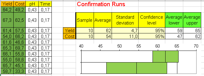
These are the confidence intervals for Yield and Cost corresponding to these ideal values of pH and Time.
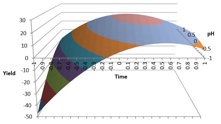
Response Surface Graphics
Since we only have two significant factors in this case (pH and Time) we can draw the response surfaces corresponding to our estimated formulas:


Photolitography Process
Let us now analyse another example.
We want to meet the following response specifications:

By adjusting the following critical factors:

So we have run Response Surface CCI experiments and added quadratic and interaction terms for the analysis (Sheet PHOTO):

The analysis results for the three responses (sheet PHOTOanalysis):

We now prepare for Solver:

For each response we only select those factors and interactions which are significant (p < 0.05)
We need Solver to calculate the values for the factors in the yellow cells (AI15-AI17)
These factor values should be between +1 and -1
We specify the max and min values required in the responses
We select response EDGE to be maximized as well as meet the min restriction of 3.
Solver was able to find factor values that meet all specifications.
Conclusions
- Design of experiments could be extended to non-linear relations between factors and responses
- In some occasions more than one response needs to be optimized
- Excel data analysis regression can be used to approximate a mathematical formula to each of the responses
- Excel Solver is useful to optimize the process, meeting multiple factor and response restrictions
- Several alternatives can be easily analysed with Solver once the mathematical model has been validated


Comments
Post a Comment