Autocorrelation: How to Manage it

When a process variable has only random variation, each output is independent of the previous ones.This is what happens in a lottery.
In some processes this independence does not happen.
If we control our daily weight, for instance, our weight today is correlated to the weight of the previous days: it has autocorrelation.

Weight Autocorrelation

Our weight today is correlated with:
The day before: 39%Yesterday's weight: 53%
Body weight has inertia: you don't expect sudden changes.
A similar effect happens when you control a heavy aircraft or a ship: its masive weight prevents you from making a sharp turning or make a sudden stop.
This opposing force to change is what is called Inertia.
This inertia definition applies to moving objects and it is proportional to the object mass.
Inertia also applies to fluids: a tank accumulating a fluid will also have this inertia effect.
If we try to control a process, which only has random variation, by reacting to every output, we can see in Dice throwing Exercise that the process will get worse: variation will increase. This is a case of over-reaction.
We will see another instance of over-reaction caused by process inertia.
Airplane Tilt Control
We will now experience how to control a process with inertia, with a simulator of the tilt control in an airplane:

Download this Excel file Inertia simulator.xlsm from OneDrive.
Close other Excels and allow macros to run it.
Press Start to start simulating.
Move the cursor Up/ Down to adjust the tilt (do not click).
You should try to keep tilt as close to zero as possible.
The graphs below will show you the adjustments you made and the actual tilt evolution along 50 runs.
The Average and StdDev on top will tell you the extent of your success: you want both to be minimal.
Tilt Reduction by Adjusting

We experienced the difficulty of reacting to this random behavior.

It is normal with an average of 1.47 and a standard deviation of 4.01.
We analyse the evolution along time with an SPC chart:


In this case there is no evidence of autocorrelation: each outcome is independent of the previous ones.
Response delay
When you try to control this process the first thing you notice is that there is a delay between your adjustments and the tilt response:

This is the result of inertia: the response is slow.
Continuous Process Balancing by Fluid Accumulation in a Tank

Pure water has a pH of 7.
In the following example accumulation in a tank has been used in order to reduce the pH standard deviation and meet the required regulations.

Tank Acumulation Effect

We can see variation has been significantly reduced.

Resulting in an average pH of 5.99 and a standard deviation of 0.42 which gives a Cpk of 1.17 (a significant improvement from 0.08)

How to Manage Autocorrelation
- It should follow a normal distribution
- Each output should be independent of the previous ones: no autocorrelation


Download this Excel file Resistivity.xlsx from OneDrive

There is significant autocorrelation.
Exponential Smoothing with Excel Solver

To do this we will calculate the transformed EWMA of RESISTIVITY:
Where LAMBDA is a number between 0 and 1
We will use Excel Solver to calculate LAMBDA to minimise the residuals in column C:
We compute the total quadratic error (sum of squares) in
Now we ask Solver to minimise the total error in E2 by calculating LAMBDA in D2 with the restrictions that it should be between 0 and 1.
Now let's see the original Resistivity and transformed EWMA in a graph:


We have now removed the false alarms from the SPC chart and keep only the real out-of-control symptoms.
Now let's check for Residuals autocorrelation:

We see no significant autocorrelation.
Conclusions
- Process inertia shows with autocorrelation: metric values are dependent of previous values
- Inertia causes a delay between action and response, which may produce over-reaction when you try to control the process
- Mechanical inertia is proportional to the mass of the object (airplane, ship).
- Fluid inertia is proportional to the volume of its storage in a tank or pond.
- A flywheel is used in a car engine to smooth rotation speed, by increasing mechanical inertia.
- Fluid accumulation in a tank is used to reduce variation.
- Body weight has autocorrelation.
- Autocorrelation could have a positive effect: it reduces standard deviation.
- To control an autocorrelated variable, it may be transformed by exponential smoothing, then we control the residuals instead of the original variable.
- All this can be done with Excel Data Analysis and Solver.


Comments
Post a Comment