Seasonal Trends Analysis with Excel

Hourly Production
We are going to analyse the hourly production data collected during one month:

Download this Excel file Trend Analysis.xlsx from OneDrive folder
Process stability

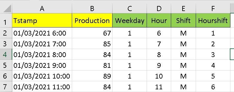
Timestamp Data Collection
Some Critical Factors we can Extract from the Timestamp
- Day of the week
- Shift
- Hour in the shift

C2 =WEEKDAY(A2;2)
D2 =HOUR(A2)
E2 =IF(D2<6;"N";IF(D2<14;"M";IF(D2<22;"A";"N")))
F2 =IF(E2="M";D2-5;IF(E2="A";D2-13;IF(D2>21;D2-21;D2+1)))
The resulting extended table is:
Day of the Week Pivot Table


Average Production Confidence Intervals

L3 =IF(I3="";"";J3-TINV(0,05;I3-1)*K3/SQRT(I3))
M3 =IF(I3="";"";J3+TINV(0,05;I3-1)*K3/SQRT(I3))
The resulting 95% confidence intervals:

We conclude that production om Mondays ( DOW = 1) is significantly lower than the other days.
We also notice that production on Fridays (DOW = 5) is significantly higher.
Maybe the two are related: The line wants to meet the weekly target on Friday and to do that it empties the line so the last process steps have nothing to work on on Monday.
With this rigorous analysis we make sure we make decisions based on data rather than impressions.
Shift Confidence Intervals
We can now do the same analysis for shifts:

Production in the night shift is significantly lower than in the other two.
Hour of the Shift Confidence Intervals

We notice a significant inefficiency at the beginning and the end of the shift. Also in the 3rd hour (maybe there is a scheduled brake).
Process With no Trends
Let us do this analysis of a manufacturing process with the same average and standard deviation but no significant trends.
First we check stability with an SPC chart:


Conclusions
- Collecting timestamps with the related data enables time based analysis
- Timestamp collection could be automatic so it doesn't add to the reporting time
- Confidence intervals enable data analysis taking into account the sample size
- Process improvement actions can be prioritized based on this analysis
- https://www.mckinsey.com/business-functions/operations/our-insights/labor-intensive-factories-analytics-intensive-productivity?cid=other-eml-dre-mip-mck&hlkid=038500d6d6644447856b60023c212207&hctky=2578305&hdpid=4439d486-774e-4fbb-8aed-02861baec336


Comments
Post a Comment