Time Variation and Lead Time Increase: A Vicious Circle
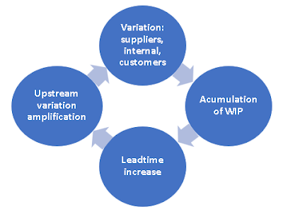
Time variation and WIP cause a vicious circle that increases value stream lead time making it difficult to keep pace with changing customer demand.
Time is a continuous variable which can be easily recorded without the need of special equipment: PCs or smartphones used to collect data can automatically record a timestamp.
When it comes to analyse cause and effect between process parameters and results time is key.
Time Variation Causes Accumulation of WIP

You can experience this effect in exercise 7 with a simulator :

This WIP Increase Causes a Lead Time Increase

As seen in the same simulator:

This is due to the fact that items have to wait in the queues formed before steps 2 and 3.
Long Lead Times Cause an Amplification Upstream of the Market Variation

This effect is well illustrated in the Beer Game which can be experienced with various simulators in the web.

The game was first described by Peter Senge in The Fifth Discipline.
A small variation in the market demand is amplified as you go upstream in the value stream, due to the long lead times, and it becomes a tsunami when it gets to the factory.
This bullwhip effect has been widely described and suffered in all sorts of distribution channels.
This obviously creates a major problem for the factory which goes through an expensive period of overtime, hiring and subcontracting.
Eventually all orders are cancelled, the whole value stream comes to a stand still and ends up with huge stocks and having to fire employees and close factories.
Variation Amplification Reinforces the Loop

It increases both variation and WIP across the value stream and therefore lead time also increases.
Unless the causes of variation are detected and reduced this problem will not be resolved.
Reducing lead time by applying Just In Time, when you have variation (exercise 8) drops throughput so deliveries will get worse.
Time Recording
When it comes to data collection in the value stream compounding data doesn't help. If we just record shift production or total number of defects it is difficult to find the cause of problems. Variation information is lost.
Nowadays it is easy to extract detailed raw data from line equipment or web applications.
On the other hand data storage has become very cheap: gigabytes for a few euros. This means it is feasible to store raw data from which we can always obtain high level reports or detailed trends and correlations.
Ideally data should be automatically collected, but this is not always possible.
If we need to collect data by hand it is essential to enter it directly into a PC, tablet or smartphone rather than use pencil and paper. This allows automatic data entry validation and eliminates the need for a manual transcription into the system at a later stage.
When data is entered directly into the system in real time you can easily, automatically, append a timestamp which will record the moment data was entered.
Rather than having to provide a terminal for each operator in order to report, an ordinary smartphone connected via WIFI to the cloud could be used. Some advantages:
- it is cheaper
- it uses an existing skill in all operators
- easier entry with voice or pull down menus
- it enables data entry validation.
Real Time Control with SPC
Statistical process control charts are used by operators to control their own process.
Data for the chart may be automatically collected or entered manually.
Feedback from an incident to the operator responsible should be quick in order to take action as soon as required.
Different SPC charts for variables or attributes can be used to avoid both over-reaction or lack of reaction on the part of the operator.

Control Plan in the Value Stream Map
A control plan includes all tests and controls established along the value stream to insure we detect defects or problems as soon as they happen.

If we just detect a defect at the end of the value stream we probably already have the defect in all the WIP from the point it was produced.
On the other hand, controls cost money and add to the lead time so the control plan should include the minimum number of controls in the most critical points.
The control plan needs to be continually adapted to the current situation to make sure it is effective and feasible.
When you have a control there is a chance that some units will fail this control, in which case you need to provide an alternative route for those items in a repair loop.This repair loop should be part of the VSM because it could eventually become a bottleneck for the total VSM
Use of Timestamp in Data Analysis
If we record the timestamp as we collect the data this could become very useful when it comes to data analysis.
We want to find out if there is a significant difference between the different days of the week and between the 3 shifts.

From the timestamp we extract the day of the week (DOW) with a formula. We also extract the hour and from this the Shift.
The result of the analysis with a two factor ANOVA is:

There are significant differences between shifts and between days of the week.
Thursdays and Fridays are the most productive and Mondays the least. Maybe it's because we start with an empty line on Mondays.
We have been able to do this analysis thanks to the timestamp recording.
Delayed Effect
We want to find the relationship between a process variable X and the output Y so we have collected data for a week every 30 minutes:

Doing a correlation analysis we obtain:

We suspect a delay between the moment X is recorded and the output Y so we will look for a correlation with delays of 30 minutes:

We now look for the correlation coefficients:

We now see a good correlation between X and Y + 5 (Y delayed 5 periods)
This means there is a delay of 5 periods (2 hours 30 minutes) between X and output Y.
Doing a regression analysis we obtain the regression line:

Conclusions
- Time variation coming from suppliers, the internal process or customers cause an accumulation of WIP in the value stream
- This accumulation of WIP causes waiting times in front of every queue
- These waiting times increase the overall lead time
- Customers expect shorter and shorter lead times
- Long lead times with variation also cause late customer deliveries: missed commitments
- Reducing lead time by applying Just In Time, when you have variation, drops throughput so deliveries will get worse
- Time variation is the root cause so it should be measured, recorded and analysed to reduce it were it is produced


Comments
Post a Comment