Minitab DOE

Optimize both Yield and Cost with Minitab Design of Experiments

Design of Experiments is a powerful technique to optimize process outputs in complex processes where multiple factors affect the outputs. When we want to optimize more than one output the problem becomes more complex.

With this example we want to follow the steps, using Minitab, to optimize both process yield and cost by acting on 3 critical factors which have been identified by previous experiments.

Process Improvement Steps

DEFINE: The first step in process improvement is to map the current process as it is really happening with a Value Stream Map.

MEASURE: Then we need to collect process data in the line.

MEASURE VARIATION: To understand the process dynamic behavior we will need statistically significant data to enable simulation   

CONTROL: The first data analysis is to check for stability with Statistical Process Control

MEASURE CAPABILITY: Once we insure the process is stable we want to know to what extent is the process able to meet the customer requirements with Process Capability

ANALYSE CRITICAL FACTORS: Confidence intervals and hypothesis testing can help in this analysis and regression to identify critical factors

IMPROVE CAPABILITY: When we identify a critical process variable that doesn't meet the capability requirements we can use Design of Experiments (DOE) to improve capability by acting on factors affecting this variable. This is what we will cover next.

Experiment Design

Based on the current values used for the three factors we decide the levels we want to experiment.

These are the factors and levels we have decided to experiment with:

  

Factorial Experiment

We will start with a full factorial experiment with 2 central points:



  

The resulting design is:

Run the Experiments

We are going to use a simulator in Excel to perform the experiments

Download this Excel simulator YieldCost.xlsx from OneDrive 

We will just copy columns C5 - C7 from Minitab to the corresponding factor columns in the simulator:



We now copy the results of the experiments (columns Yield and Cost) back to the Minitab sheet in C8 - C9:

Analyse the Results

Now we start to analyze these results of our factorial experiment with Minitab:

These are the results for Yield:



This is telling us the factorial model is not valid: R-sq(adj) is very low (9,55%). This is the proportion of variability explained by this factorial mathematical model.

If we look at the p-values none of the factors or their interactions are significant.

We suspect curvature in spite of its p-value being slightly above 0,05.

Why is the Factorial Model not Valid in this Case?

To confirm curvature we can look at the graphs of main effects both for Yield and Cost:





This, clearly, shows curvature both for Yield and Cost because the Center points are totally out of line with the Corner points.

To further confirm curvature we repeat the factorial analysis including central points:



By including the central points in the model R-sq(adj) has improved a lot (97,97%) so this confirms we need quadratic terms in the formula but these can not be calculated with a factorial experiment. 

This confirms the fact that a linear mathematical model is unable to represent our process. We need a more complex model including quadratic terms. We will try with a Response Surface set of experiments.

 

Response Surface Experiments

It is possible to use the factorial experiments we have already performed and define them as a block of cube points and just run another block of experiments with the axial points to complete the response surface set of experiments.

We are going to run a new full set of experiments for response surface in this case.

We design a Response Surface experiment with the default values for 3 factors: 1 block of 20 runs with the default number of center points.



But be aware that we must define our factor values as Axial points to avoid physically impossible values such as a negative pH.

  

The resulting response surface design is:

Run the Response Surface Experiments

To run the experiments we copy columns C5-C7 to our simulator:



And back the results of the experiments (Yield and Cost) to the new Minitab worksheet:

Analysis of the Response Surface Results

We now perform the analysis of the Response Surface Design:

With the following results for Yield:



R-sq(adj) value of 96,85% confirms the validity of this model. Also all the p-values below 0.05. Only the Temperature*Time interaction and Temperature^2 are not significant. Before we remove these from the model we must make sure they do not significantly affect the other output variable (Cost) we try to optimize:

Reduced Model

Now we confirm that both Temperature^2 and Temperature*Time do not,significantly, affect Yield or Cost.

Therefore we will remove both from the model:



The resulting reduced model for Yield is then:





This is the formula to estimate Yield as a function of Temperature, Time and pH.

The reduced model for Cost is:

Graphical Representation of the Response Surface Model

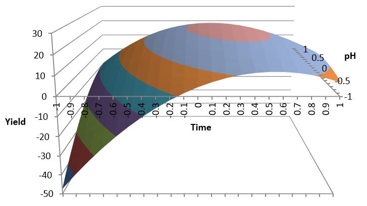
We can now see graphically the impact of the 3 factors in Yield with Contour Plots:



And also for Cost:




We can, graphically, see the optimal areas to maximize Yield and to minimize Cost. Unfortunately these areas do not coincide.

 

Optimal Factor Values Calculation

Now we will let Minitab calculate the optimal factor values to achieve our overall optimization:

We have decided to assign double weight to Yield Vs Cost. The result is:



This gives us the optimal factor settings to obtain a predicted Yield of 156 and a Cost of 97.

The following interactive graph lets us touch up the factors and see the results of both outputs:




The optimal factor values have been obtained by maximizing the Composite Desirability curves which are based on our condition that Yield is twice as important as Cost.

 

Maximize Yield at any Cost

If we wanted to maximize Yield at any Cost we would obtain:



This improves Yield but it also increases cost.

With this example you can experience the power of Minitab to design and analyze experiments in order to optimize several outputs by calculating the optimal factor settings

Conclusions

• Design of Experiments (DOE) is an effective way of process optimization. 
• First we identify the critical factors that affect process outputs. 
• Then we are able to find the values of these factors that will produce the optimal outputs. 
• Very often the relation between factors and outputs in the operating region are close to linear so factorial experiments can do the job. 
• In those cases where these relations are not linear we will need to use Response Surface Experiments (more runs) to come up with a more complex mathematical model with quadratic terms.
• Minitab is a useful application both to design the experiments and analyse the results

Alternative approach with Excel:

• Design of Experiments with Excel
• Response Surface Design of Experiments with Excel
• The Catapult exercise